Branch and Bound (BB) is a general method for finding optimal solutions to problems, typically discrete problems. A branch-and-bound algorithm searches the entire space of candidate solutions, with one extra trick: it throws out large parts of the search space by using previous estimates on the quantity being optimized. The method is due to Ailsa Land and Alison Doig, who wrote the original paper in 1960: “An automatic method of solving discrete programming problems.”
Typically we can view a branch-and-bound algorithm as a tree search. At any node of the tree, the algorithm must make a finite decision and set one of the unbound variables. Suppose that each variable is only 0-1 valued. Then at a node where the variable
 is on-tap, the algorithm must decide whether or not
  or
or  is the right choice. In a brute-force search both choices would be examined.
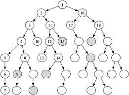
|
| src |
will lead to a value for the optimization quantity of at most  , while setting will lead to a value for this quantity of at least
  . If
. If  , then there is no reason to even consider setting to
  . The upper bound on and a lower bound on allows the algorithm to safely avoid searching a whole chunk of the space: all those cases where would be set to . This is the power of the method.
 Search Time and Branching Factor
In many practical cases, the amount of pruning that occurs in this type of BB algorithm can be immense. This in short is why the algorithm can be so powerful. This is often expressed via the effective branching factor (EBF): the number so that your search took the same time as searching an -ary tree with no pruning. If you are searching a tree of depth
  , this is well-defined as the -th root of the total number of nodes you searched.
For example, suppose you have the above binary tree and get the “
 ” savings half the time. You might think that means on average you expand
  children, so
  , but this is wrong in both directions. Consider a binary tree where you get the
savings at every node in the level above the bottom. Since about half
the nodes are in the bottom level, you could say you searched
, but this is wrong in both directions. Consider a binary tree where you get the
savings at every node in the level above the bottom. Since about half
the nodes are in the bottom level, you could say you searched  not
not  nodes, so your EBF is
 ^{1/d} = 2^{1 - 1/d}}") which is scarcely different from
which is scarcely different from  .
.Suppose instead that you get the savings at every other level in the binary tree. Then you have branching at only half the levels, so it is as if you searched a whole tree of depth
 . There is an issue of
being odd or even, which matters but not hugely, since pruning the
bottom layer is not so valuable. So we may estimate the number of nodes
searched as
. There is an issue of
being odd or even, which matters but not hugely, since pruning the
bottom layer is not so valuable. So we may estimate the number of nodes
searched as  . Now the EBF is
  which beats
  . Generally for an
  -ary tree this pruning pattern gives an EBF of
  .
.One way to express the issue of upper and lower bounds for BB is, can we give upper and lower bounds on the EBF? This is only a rough way to estimate the time, but already it is hard to do.
Why So Hard To Understand?
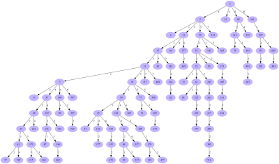
I think the reason that BB algorithms are so hard to prove bounds lower or upper is that they fall into a category of sequential algorithms. Of course all algorithms can be viewed as sequential—this was the source of discussion with Nemirovski, I believe. But what I mean is an algorithm that moves from state to state in a manner that is complex, in a manner that does not seem to follow any obvious path. People who have played complex games like chess can recall times when the path was especially hard to find.I am not explaining this well, perhaps because the notion is unclear in my mind. But here is an analogy with another problem. Consider the famous Collatz conjecture, named after Lothar Collatz, who first proposed it in 1937.
Take any natural number n. If n is even, divide it by 2 to get n/2. If n is odd, multiply it by 3 and add 1 to obtain 3n + 1. Repeat the process. The conjecture is that no matter what number you start with, you will always eventually reach 1.Paul Erdős said, allegedly, about the this conjecture:
“Mathematics is not yet ripe for such problems.”There is something inherently sequential that makes them impossible for us, right now, to understand. I think the same behavior is at work with BB algorithms.
|
| source for Collatz tree |
Is There a General “Proof Method”?
Ken thinks there are two reasons, one merely cultural and the other intractable—basically reflecting my reason. The cultural one is that the depth is usually polynomially related to what is considered the size “ ”
of the problem. For instance, while trying to solve a
traveling-salesman or clique problem the depth is the size of the graph.
Any EBF
”
of the problem. For instance, while trying to solve a
traveling-salesman or clique problem the depth is the size of the graph.
Any EBF  makes
makes  an exponential function of .
This is an immediate cut-off from polynomial-time algorithms, so Ken
thinks this theoretical space has not been searched as well as it could
be.
an exponential function of .
This is an immediate cut-off from polynomial-time algorithms, so Ken
thinks this theoretical space has not been searched as well as it could
be.Ken’s main reason is that branch-and-bound methods always have some ad-hoc ingredients: the means of proving bounds on the quantity being optimized. The metric is usually clear, such as the cost of a tour or the size of a clique or the value of a chess position, but the means are not. The problem domain must be taken into account, especially what kind of regularities it enjoys. Other factors may be involved that enable greater savings even than bounds that have been theoretically “proved” in general. Two relevant instances are chess engines and Rubik’s Cube®.
One Fish, Two Fish…
Essentially all strong chess-playing programs are based on alpha-beta search. Two top programs now are Rybka, which is Polish for “little fish,” and Stockfish, of Norwegian roots like Magnus Carlsen, who just set the all-time (human) rating record. A “fish” usually means a poor player, but these programs seem not to mind.Here’s the basic idea of alpha-beta: Suppose Alice and Bob are playing chess, and Alice has found that move
 has a value of
  = 2}") and is now searching a possible alternative move
and is now searching a possible alternative move  . Suppose the first possible move
  Bob can make in reply to gives value . So we know already
  \leq 0}") , so move is already proved to be sub-optimal for Alice. What we save by pruning is having to look at Bob’s other moves
, so move is already proved to be sub-optimal for Alice. What we save by pruning is having to look at Bob’s other moves  for
for  . Note that this savings depends not only on hitting upon a good move by Bob early, but also on having tried one of Alice’s best moves first.
 Even if we make the best initial tries, for Bob’s
we still have to consider all of Alice’s possible next-moves  in order to be sure that the value there is really no better than . This is like the tree case above where you save on every other level, so that the EBF is . In chess the number of legal moves is typically in the high thirties, so that gives an EBF of about 6.
Well that’s if Alice always gets lucky. If you have no advance idea about values and have an average amount of luck, a 1982 paper by Judea Pearl—winner last March of the Turing Award—calculated the average-case EBF as
 . For chess that would be about 14.
So is 6 a solid lower bound? If it were, then Garry Kasparov would never have lost to Deep Blue, and I (Ken writing this and the next two sections) wouldn’t be asked to worry about cheating with computers at chess.
…in Alpha-Beta Better Beater Battle
When faced with a need to search 8 moves ahead for each player (that’s 16 tree levels, called plies), two of the most important ideas for chess programs are don’t search 8 moves ahead and don’t move at all. First, try a “pilot search” maybe 4 or 5 moves ahead, which takes trivial time. By the regularity of move values usually not changing much at higher depths, this helps you “get lucky” with the order much of the time. It turns out that other factors favor doing all the lower-order searches ,
,  ,
,  , …,
, …,  before doing depth , a process called iterative deepening. Stockfish even outputs its results starting from
  .
.Chess programmers also employ heuristics to try to lower the effective
by flagging some moves as apparently so bad at depth  that they need not even be tried to see if they improve at depth . But the most surprising idea is not to consider any moves at all: take
  and let the opponent have two moves in a row.
This is illegal in chess but works like a charm because often Alice can thereby prove that Bob’s last move was sub-optimal as the search branch bottoms out, without having to lift a finger herself. The main hitch is that chess has a feature called Zugzwang whereby Alice passing would be an unfair advantage. But it usually happens only in endgame positions with lower
so the chess engine can throttle back on heuristics. It’s the opposite of the Red Queen saying to Alice,“Now, here, you see, it takes all the running you can do, to keep in the same place.”Instead, in chess programs, Alice often progresses best by not moving. This null-move idea takes the most basic assumption one might make about expanding nodes in a lower-bound proof, and knocks it off the board.
Some chess engines prefer other tricks, and there are other tradeoffs—indeed the tricky position covered here induced one commercial programmer to change his pruning strategy (he called it a bug-fix and thanked me). While alpha-beta itself is always worst-case correct, these other ideas take some risks. But the upshot is that EBF’s under 2.5 are routinely achieved. The engines battle over decrements of 0.1 or even 0.01 in the EBF, but they’re significant because they’re in the base of an exponent.
Proofs and Rubik’s Cube
Well chess is not a simple case of branch and bound because it alternates minimizing and maximizing, and because many heuristics compromise correctness. Let’s consider Rubik’s Cube, a nice finite problem where the number of legal ‘moves’ is the same in every position, the search has a clear goal, and the only quantity being minimized is the length of the path to that goal. A 180-degree rotation counts as one move. It is literally child’s play—kids have solved random cases in under 10 seconds.There are exactly
 positions to search, so clearly brute-force is out of the question.
Enter BB and several other ideas. Only recently in 2010 was it proved that every position can be solved in 20 or fewer moves. This Wikipedia page also documents the improvements in bounding the value. How were they achieved?
positions to search, so clearly brute-force is out of the question.
Enter BB and several other ideas. Only recently in 2010 was it proved that every position can be solved in 20 or fewer moves. This Wikipedia page also documents the improvements in bounding the value. How were they achieved? 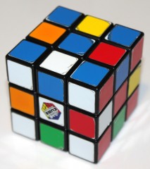
|
| source for 20-move “superflip” position |
 moves have been made, and a quick-check shows that the links demand
more moves than the goal figure allows, the search can be cut off there.
Of course algebra rules the Rubik problem structure, so did this
produce the best proof? No, it gave an upper bound of 52, later improved
only to 40.
moves have been made, and a quick-check shows that the links demand
more moves than the goal figure allows, the search can be cut off there.
Of course algebra rules the Rubik problem structure, so did this
produce the best proof? No, it gave an upper bound of 52, later improved
only to 40.In 1997 Richard Korf applied a whole new search method called IDA* which he had invented in 1985. Instead of subgroups he identified “sub-cubes”—sub-problems that had to be solved along with the main one—that were more ad-hoc than the group decomposition. He also applied iterative deepening like a chess engine, and got … only a bunch of random cases solved within 18 moves. We now know that over 95% of positions are solvable within 18 moves, over 67% needing 18 as well. His was a better algorithm in action, but it didn’t prove an upper or lower bound.
The optimal solvers went back to the group structure, but pre-packaged the use of symmetry in a different way, and found ways to fit needed portions of the search space into separate chunks within the memory of the computers that Google allowed them to use. This still took the equivalent of 35 years of time on a standard 2.8Ghz quad-core CPU.
Is there a general principle for proving good upper and lower bounds, either on solution quality or on time of search, even for a simple well-structured problem like Rubik’s Cube? That would seem a pre-req for any general theory of understanding branch-and-bound.
No comments:
Post a Comment