STACK Memory

Let's look at the following example and see how the local variables are set in the stack area:

void f1()
{
 int a;
 short b[4];
 double c;
 f2();
 f3();
} 

When we call f1() function, space needs to be set aside. The following picture shows activation records/stack frame:

 

When the function f1() is called, the stack pointer will be decremented by 20 bytes which is the size of the variables of f1().

 

void f2()
{
 int x;
 char *y;
 char *z[2];
 f3();
}

void f3()
{
 double m[3];
 int n;
}

The following diagram shows the movement of stack pointer, sp: f1()->f1.f2()->f2.f3()->f2.f3() exits->f1.f2() exits.

After the f1.f2(), when we call f1.f3(), the variables of the function f3() simply overwrites them onto the area where the variables of f2() were.

HEAP MEMORY

Heap memory, also known as dynamic memory, is an alternative to local stack memory. Local memory is so automatic that it is allocated automatically on function call and it is deallocated automatically when a function exits. Heap memory is different in every way. The programmer explicitly requests the allocation of a memory block of a particular size, and the block continues to be allocated until the programmer explicitly requests that it be deallocated. Nothing happens automatically. So the programmer has much greater control of memory, but with greater responsibility since the memory must now be actively managed.

The advantages of heap memory:

• Lifetime:
  Because the programmer now controls exactly when memory is allocated and deallocated, it is possible to build a data structure in memory, and return that data structure to the caller. This was never possible with local memory which was automatically deallocated when the function exited.
• Size:
  The size of allocated memory can be controlled with more detail. For example, a string buffer can be allocated at run-time which is exactly the right size to hold a particular string. With local memory, the code is more likely to declare a buffer size 1000 and hope for the best.

The disadvantages of heap memory:

• More Work:
  Heap allocation needs to be arranged explicitly in the code which is just more work.
• More Bugs:
  Because it's now done explicitly in the code, realistically on occasion the allocation will be done incorrectly leading to memory bugs. Local memory is constrained, but at least it's never wrong.

However, there are many problems that can only be solved with heap memory, so that's that way it has to be. In languages with garbage collectors such as LISP and Java, the above disadvantages are mostly eliminated. The garbage collector takes over most of the responsibility.

HEAP ALLOCATION

The heap is a large area of memory available for use by the program. The program can request blocks of memory for its use within the heap. In order to allocate a block of some size, the program makes an explicit request by calling the heap allocation function. The allocation function reserves a block of memory of the requested size in the heap and returns a pointer to it.

Suppose a program makes three allocation requests to 25 allocate memory to hold three separate images in the heap each of which takes 1024 bytes of memory.

Each allocation request reserves a contiguous area of the requested size in the heap and returns a pointer to that new block to the program. Since each block is always referred to by a pointer, the block always plays the role of an object that the pointer can points to and the program always manipulates its heap blocks through pointers. The heap block pointers are sometimes known as base addresspointers since by convention they point to the base, lowest address byte, of the block.

In this example, the three blocks have been allocated contiguously starting at the bottom of the heap, and each block is 1024 bytes in size as requested. In reality, the heap manager can allocate the blocks wherever it wants in the heap so long as the blocks do not overlap and they are at least the requested size. At any particular moment, some areas in the heap have been allocated to the program, and so are in use. Other areas have yet to be committed and so are free and are available to satisfy allocation requests. The heap manager has its own, private data structures to record what areas of the heap are committed to what purpose at any moment The heap manager satisfies each allocation request from the pool of free memory and updates its private data structures to record which areas of the heap are in use.

HEAP DEALLOCATION

When the program is finished using a block of memory, it makes an explicit deallocation request to indicate to the heap manager that the program is now finished with that block.

The heap manager updates its private data structures to show that the area of memory occupied by the block is free again and so may be reused to satisfy future allocation requests.

After the deallocation, the pointer continues to point to the now deallocated block. The program must not access the deallocated object. The pointer is there, but it must not be used. Sometimes the code will set the pointer to NULL immediately after the deallocation to make explicit the fact that it is no longer valid.

HEAP - SUMMARY

• The heap is an area of memory available to allocate blocks of memory for the program.
• There is some heap manager library code which manages the heap for the program. The programmer makes requests to the heap manager, which in turn manages the internals of the heap. In C, the heap is managed by the ANSI library functions malloc(),free(), and realloc().
• The heap manager uses its own private data structures to keep track of which blocks in the heap are free and which blocks are currently in use by the program and how large those blocks are. Initially, all of the heap is free.
• The heap may be of a fixed size, or it may appear to be of a fixed but extremely large size backed by virtual memory. In either case, it is possible for the heap to get full if all of its memory has been allocated and so it cannot satisfy an allocation request. The allocation function will communicate this runtime condition in some way to the program - usually by returning a NULL pointer or raising a language specific runtime exception.
• The allocation function requests a block in the heap of a particular size. The heap manager selects an area of memory to use to satisfy the request, marks that area as in use in its private data structures, and returns a pointer to the heap block.
  The caller is now free to use that memory by dereferencing the pointer. The block is guaranteed to be reserved for the sole use of the caller - the heap will not hand out that same area of memory to some other caller. The block does not move around inside the heap - its location and size are fixed once it is allocated.
  Generally, when a block is allocated, its contents are random. The new owner is responsible for setting the memory to something meaningful. Sometimes there is variation on the memory allocation function which sets the block to all zeros (calloc() in C).
• The deallocation function is the opposite of the allocation function. The program makes a single deallocation call to return a block of memory to the heap free area for later reuse. Each block should only be deallocated once. The deallocation function takes as its argument a pointer to a heap block previously furnished by the allocation function. The pointer must be exactly the same pointer returned earlier by the allocation function, not just any pointer into the block. After the deallocation, the program must treat the pointer as bad and not access the deallocated object.

NEED A COPY CONSTRUCTOR

Let's look at the following example:

#include <iostream>

using namespace std;

class Student 
{
public:
 int id;
 char *name;
 Student() 
 {
  id = 0;
  name = "";
 }
};

int main() 
{
 Student student1;
 student1.id = 10;
 char nm[] = "Clinton";
 student1.name = nm;

 Student student2 = student1;
 student2.name[0] = 'P';
 cout << student1.name; // Plinton
 return 0;
}

As shown in the example, we made another instance of Student class which is student2 from an existing instance student1. However, later we modified an element of the name array. It turned out that modifying a field of one instance can affect the other instance, and that's not we wanted.

So, to control the assigning operation, we need our own copy constructor not the default copy constructor that compiler provides:

#include <iostream>

using namespace std;

class Student 
{
public:
 int id;
 char *name;
 Student() 
 {
  id = 0;
  name = "";
 }

 Student(Student &s)
 {
  id = s.id;
  name = strdup(s.name);
 }
};

int main() 
{
 Student student1;
 student1.id = 10;
 char nm[] = "Clinton";
 student1.name = nm;

 Student student2 = student1;
 student2.name[0] = 'P';
 cout << student1.name << endl; // Clinton
 cout << student2.name << endl; // Plinton
 return 0;
}

Note that strdup() in our own copy constructor does dynamic memory allocation for the character array including the end character '\0' and returns the address of the heap memory. In other words, the new instance has its own memory to store the name not shared one with which it was instantiated from.

MATLAB TUTORIAL : INDEXING & MASKING

ACCESSING INDIVIDUAL ELEMENTS

>> M = [1 2 3; 4 5 6; 7 8 9]
M =  1     2     3
     4     5     6
     7     8     9

We can access individual element by specifying (row, column):

>> M(2,3)
     6

Also, note that Matlab is using 1-based index not 0-based index.

SLICING ARRAYS

>> 1:4
ans =
     1     2     3     4

We can take a portion of matrix using slice.

>> M = [1:20]
>> M2 = reshape(M,4,5)
     1     5     9    13    17
     2     6    10    14    18
     3     7    11    15    19
     4     8    12    16    20
>> M2(1:4, 3:4)
     9    13
    10    14
    11    15
    12    16

We took all rows and 3rd and 4th columns.

When we takes all rows or columns, we don't have to use specific indices, and we can use this form:

>> M2(:,3:4)
     9    13
    10    14
    11    15
    12    16

SHIFTING DATA USING SLICE

The following example assigns value of the last three element to the first three elements:

>> v = 10:10:100
    10    20    30    40    50    60    70    80    90   100

>> v(1:3) = v(8:10)
    80    90   100    40    50    60    70    80    90   100

ARRAY AS SUBSCRIPTS

>> a = 10:10:100
    10    20    30    40    50    60    70    80    90   100

>> index = [1 10 5 7 9]
     1    10     5     7     9

>> b = a(index)
    10   100    50    70    90

In the code, we made a new array by using array as subscripts to the source array.

COMPARISON

We can compare each element with a value, and the output is a type of boolean not double:

>> a = 1:10
    1     2     3     4     5     6     7     8     9    10

>> b = a < 7
     1     1     1     1     1     1     0     0     0     0

We can use this to make another array:

>> new_a = a(a<7)
     1     2     3     4     5     6

The operation only takes elements that a<7 is true. Since we have a new array b, we can get the same result by doing this:

>> new_a = a(b)
     1     2     3     4     5     6

However, we cannot do this:

>> b2 = [1 1 1 1 1 1 0 0 0 0]
     1     1     1     1     1     1     0     0     0     0

>> new_a2 = a(b2)
Subscript indices must either be real positive integers or logicals.

That's because the elements of b2 is not a boolean but a double type.

ASSIGNING USING A MASK

We can assign a value to only an element that the mask has true value:

>> a = [0 1 2 3];
>> mask = [true false true false];
>> a(mask) = [100 102]
a =
   100     1   102     3

USING MASK WHILE KEEPING THE ARRAY SIZE

Let's see how the masking changes the size of an array:

>> a = 0:10:100
     0    10    20    30    40    50    60    70    80    90   100

>> mask = a < 80
     1     1     1     1     1     1     1     1     0     0     0

>> a(mask)
     0    10    20    30    40    50    60    70

But we want to keep the size of an array unchanged while we can still applying the mask. We can achieve this by using dot(.) meaning every element:

>> a.*mask
     0    10    20    30    40    50    60    70     0     0     0

What it is doing is a element-wise multiplication with the mask!

MATLAB TUTORIAL - M FILES (SCRIPTS)

M-FILES

M-files are macros of MATLAB commands. The M-files are stored as ordinary text files with the extension m, filename.m. An M-file can be either a function with input and output variables or a list of commands.

WHERE?

Where should we put the M-files?

MATLAB requires that the M-file must be stored either in the working directory or in a directory that is specified in the MATLAB path list.

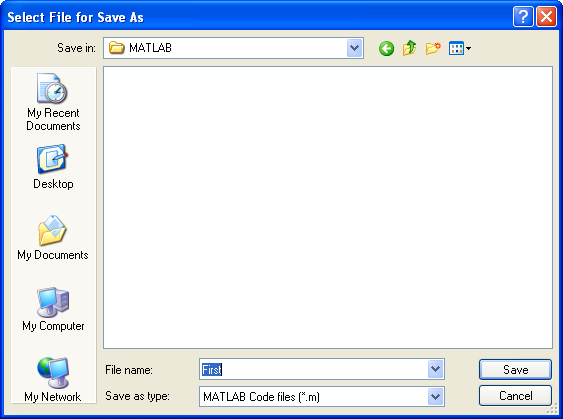
On Windows, the default location is C:\Documents and Settings\user\My Documents\MATLAB. We can check it by New->Scriptand then Save As:

 

SPECIFYING M-FILES DIRECTORY

Suppose we want to have the M-files in C:\Documents and Settings\user\My Documents\MATLAB\FFT. We can let Matlab know where it can find the file in two ways:

1. Change the working directory by issuing cd path command:

   >> pwd
   ans =
   C:\Documents and Settings\admin\My Documents\MATLAB
   >> cd FFT
   >> pwd
   ans =
   C:\Documents and Settings\admin\My Documents\MATLAB\FFT
   

2. Add the directory to the path.
   • Permanent addition to the path : edit the ....\MATLAB\matlabrc.m file
   • Temporary modification to the path : issue a command, path(path,'C:\Documents and Settings\user\My Documents\MATLAB\FFT') withing Matlab

A FUNCTION DEFINED IN M-FILE

In this section, we'll see how the M-files are used.

Let's create a file in our working directory (the default directory mentioned in previous section). Name it as cexp.m that has the following commands:

function fval = cexp(a,b)
fval = exp(a+b*i)

Then within the command window:

>> x = 1;
>> y = 2;
>> cexp(x,y)
fval =
  -1.1312 + 2.4717i
ans =
  -1.1312 + 2.4717i
>> 

MATLAB TUTORIAL : VECTORS AND MATRICES

VECTORS

MATLAB is based on matrix and vector algebra. So, even scalars are treated as 1×1 matrices.

We have two ways to define vectors:

1. Arbitrary element (not equally spaced elements):
   

   >> v = [1 2 5];
   

   This creates a 1×3 vector with elements 1, 2 and 5. Note that commas could have been used in place of spaces to separate the elements, like this:

    
   >> v = [1, 2, 5];
   

   Keep in mind that we the index of the first element is 1 not 0:
   

   >> v(0)
   Subscript indices must either be real positive integers or logicals.
   >> v(1)
   ans =
        1
   

   If we want to add more elements:
   

   >> v(4) = 10;
   

   The yields the vector v=[1,2,5,10].
   We can also use previously defined vector:
   

   >> >> w = [11 12];
   >> x = [v,w]
   

   Now, x=[1,2,5,10,11,12,]
2. Equally spaced elements :

   >> t = 0 : .5 : 3
   

   This yields t=[0 0.5000 1.0000 1.5000 2.0000 2.5000 3.0000] which is a 1×7 vector. If we give only two numbers, then the increment is set to a default of 1:
   

   >> t = 0:3;
   

   This will creates a 1×4 vector with the elements 0, 1, 2, 3.

One more, adding vectors:

>> u = [1 2 3];
>> v = 4 5 6];
>> w = u + v
w =
     5     7     9

COLUMN VECTORS

We can create column vectors. In Matlab, we use semicolon(';') to separate columns:

>> RowVector = [1 2 3]   % 1 x 3 matrix
RowVector =
     1     2     3

>> ColVector = [1;2;3]   % 3 x 1 matrix
ColVector =
     1
     2
     3

>> M = [1 2 3; 4 5 6]    % 2 x 3 matrix

M =

     1     2     3
     4     5     6

MATRICES

Matrices are defined by entering the elements row by row:

>> M = [1 2 3; 4 5 6]
M =
     1     2     3
     4     5     6

There are a number of special matrices:

null matrix	M = [ ];
mxn matrix of zeros	M = zeros(m,n);
mxn matrix of ones	M = ones(m,n);
nxn identity matrix	M = eyes(n);

If we want to assign a new value for a particular element of a matrix (2nd row, 3rd column):

M(2,3) = 99;

ACCESSING MATRIX ELEMENT

We can access an element of a matrix in two ways:

• M(row, column)
• M(n-th_element)

>> M = [10 20 30 40 50; 60 70 80 90 100];
>> M
M =
    10    20    30    40    50
    60    70    80    90   100
 
>> M(2,4) % 2nd row 4th column
ans =
    90

>> M(8)  % 8th element 10, 60, 20, 70, 30, 80, 40, 90...
ans =
    90

Also, we can access several elements at once:

>> M(1:2, 3:4)  % row 1 2, column 3 4
ans =
    30    40
    80    90
>> M(5:8)   % from 5th to 8th elements
ans =
    30    80    40    90

ELEMENT BASED OPERATION USING DOT('.')

If we use dot('.') on an operation, it means do it for all elements. The example does ^3 for all the elements of a matrix:

>> M = [1 2 3; 4 5 6; 7 8 9];
>> M
M =
     1     2     3
     4     5     6
     7     8     9

>> M.^3
ans =
     1     8    27
    64   125   216
   343   512   729

We can get inverse of each element:

>> 1./M
ans =
    1.0000    0.5000    0.3333
    0.2500    0.2000    0.1667
    0.1429    0.1250    0.1111

INVERSE MATRIX

We get inverse of a matrix using inv():

>> M = [1 2; 3 4]
M =
     1     2
     3     4

>> inv(M)
ans =
   -2.0000    1.0000
    1.5000   -0.5000

TRANSPOSE MATRIX USING A SINGLE QUOTE(')

We get transpose of a matrix using a single quote("'"):

>> M = [1 2 3; 4 5 6; 7 8 9]
M =
     1     2     3
     4     5     6
     7     8     9

>> M'
ans =
     1     4     7
     2     5     8
     3     6     9

FLIPUD() AND FLIPLR()

flipud(): flip up/down:

>> M = [1 2 3; 4 5 6; 7 8 9]
M =
     1     2     3
     4     5     6
     7     8     9

>> flipud(M)
ans =
     7     8     9
     4     5     6
     1     2     3

fliplr(): flip left/right:

>> M
M =
     1     2     3
     4     5     6
     7     8     9

>> fliplr(M)
ans =

     3     2     1
     6     5     4
     9     8     7

ELEMENT ROTATION

We can do rotate elements, for instance, 90 degree counter-clock wise:

>> M

M =

     1     2     3
     4     5     6
     7     8     9

>> rot90(M)

ans =

     3     6     9
     2     5     8
     1     4     7

RESHAPE()

We can make a change to the number of rows and columns as far as we keep the total number of elements:

>> M = [1 2 3 4; 5 6 7 8; 9 10 11 12]
M =
     1     2     3     4
     5     6     7     8
     9    10    11    12

>> reshape(M, 2, 6)  % Convert M to 2x6 matrix
ans =
     1     9     6     3    11     8
     5     2    10     7     4    12

VECTOR & FUNCTION

Functions are applied element by element:

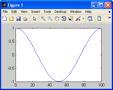
>> t = 0:100;
>> f = cos(2*pi*t/length(t))
>> plot(t,f)

f=cos(2πt/length(t)) creates a vector f with elements equal to 2πt/length(t) for t=0,1,2,...,100.