Thursday, December 28, 2023

NP Complete Class

Introduction

One of the - confusing - topics in Algorithm design is the concept of NP completeness. If you search the topic on the internet you will probably find tons of articles and lectures on the subject however in this short article I will summarize it so that it is easy to remember by the average student or software engineer.

It is all about Running Time

Computational complexity analysis refers to the study of computer algorithms in terms of efficiency. Given a problem of some input size, we need to know how fast or slow it runs as the input size grows to large values. Consider the following examples:

·      Looking an item up in a perfect hash table takes a constant time, theoretically speaking, no matter how big the hash table is, the item can be found instantly (assuming it exists), the algorithm is said to have a running time of O(1). This is indeed very fast.

·      The running time to look up an item in a sorted binary search tree of (n) elements is O(Log(n)) for example if the number of items is (32) then the number of comparisons needed to find an element is (5) in the worst case. As you can see this is a fast algorithm

·      Searching for an element in an unsorted array runs in linear time O(n). If the array contains 100 elements then you need to make 100 comparisons to find the element in the worst case. This means, the algorithm will slow down linearly as the input size grows. To be exact, the running time linearly grows as the input size becomes larger.

Polynomial versus Exponential

Algorithms with a running time function of the form O(n^k) where (k) is a constant are said to run (or solved) in polynomial time. Theoretically speaking, they are fast even if (k) is large. On the other hand, algorithms with a running time of the form O(k^n) where (k) is a constant are said to run in exponential time. These algorithms are very slow. Actually it may take a computer years to finish running the algorithm.

P, NP, NP-Complete, NP-Hard

Now we know what running time means, based on that we can classify problems into classes depending on how complex they are. I will be using plain English as opposed to mathematical terms in order to make it easy to understand.

P Problem

P means that there exists an algorithm to solve the problem which runs in polynomial time. If you are still not sure what running time or polynomial means then please read the introduction one more time.

NP Problem

NP problem means that there exists an algorithm to verify a given solution is correct in polynomial time. Note that we are talking about solution verification. We are not talking about the solution for the problem because no one has ever yet discovered a fast (polynomial) solution for NP problems nor proved the solution does not exist in the first place. NP does not mean None Polynomial, please do not say that in front of people because it is embarrassing, NP stands for non deterministic which means the problem can be solved in polynomial time BUT using none deterministic machine (of course it is not the regular computer we use every day, this computer is in the mind of some weird computer scientists. If you are interested you can research it on your own. Try to search for Turing Machine)

NP-Hard Problem

Now we know what NP means, NP-Hard problem is AT LEAST as hard as any NP problem. It could be harder, who knows. Again, when thinking about problem difficulty we are still referring to the running time of the algorithm. A harder problem takes more time to finish running.

Reduction

It feels bad when you try to solve a problem and it turns to be very hard to the extent that many people have tried it without success. In order to claim that the problem cannot be solved by many people then you need to prove that it is equivalent to some known hard problem. Reduction refers to transforming a problem to another well known (hard) problem so that people won’t dare to call you stupid.  This conversion process should run in polynomial time and can be used to prove a problem is NP-Complete as we will indicate later.

NP-Complete Problem

NP-Complete problem is both NP and NP-Hard. You know what NP and NP-Hard means, so NP-Complete means a problem that is easy to verify a given solution and every problem in NP can be reduced to our problem. The hard part is proving the first example of an NP-complete problem but our friend Steve Cook did that in the 1970s. Thanks to him because he did a great job so that we are not called stupid. In few words, in order to prove that a given problem is NP-Complete then

·      Show it is NP: given a solution, show that it can be verified in polynomial time

·      Show it is NP-Hard: pick an already known NP-Complete problem and show that you can reduce it back to our problem in polynomial time

What is the big deal about the question P = NP?

·      If P is the same as NP then this is good news, there are many interesting real life problems that could be solved very quickly.

·      It is going to be really embarrassing for the folks working in computer science field because it is believed (I am assuming someone got the $1000000 prize) for long time by many people that they are not the same.

·      In reality many believe they are not the same because many people knocked their heads against the wall for so long without any success and because crazy scientists need a proof a solution does not exist, it is going to be an open question.


Thursday, November 30, 2023

Complexity and Big-O Notation

An important question is: How efficient is an algorithm or piece of code? Efficiency covers lots of resources, including:
  • CPU (time) usage
  • memory usage
  • disk usage
  • network usage
All are important but we will mostly talk about CPU time in 367. Other classes will discuss other resources (e.g., disk usage may be an important topic in a database class).
Be careful to differentiate between:
  1. Performance: how much time/memory/disk/... is actually used when a program is run. This depends on the machine, compiler, etc. as well as the code.
  2. Complexity: how do the resource requirements of a program or algorithm scale, i.e., what happens as the size of the problem being solved gets larger.
Complexity affects performance but not the other way around.
The time required by a method is proportional to the number of "basic operations" that it performs. Here are some examples of basic operations:
  • one arithmetic operation (e.g., +, *).
  • one assignment
  • one test (e.g., x == 0)
  • one read
  • one write (of a primitive type)
Some methods perform the same number of operations every time they are called. For example, the size method of the List class always performs just one operation: return numItems; the number of operations is independent of the size of the list. We say that methods like this (that always perform a fixed number of basic operations) require constant time.
Other methods may perform different numbers of operations, depending on the value of a parameter or a field. For example, for the array implementation of the List class, the remove method has to move over all of the items that were to the right of the item that was removed (to fill in the gap). The number of moves depends both on the position of the removed item and the number of items in the list. We call the important factors (the parameters and/or fields whose values affect the number of operations performed) the problem size or the input size.
When we consider the complexity of a method, we don't really care about the exact number of operations that are performed; instead, we care about how the number of operations relates to the problem size. If the problem size doubles, does the number of operations stay the same? double? increase in some other way? For constant-time methods like the size method, doubling the problem size does not affect the number of operations (which stays the same).
Furthermore, we are usually interested in the worst case: what is the most operations that might be performed for a given problem size (other cases -- best case and average case -- are discussed below). For example, as discussed above, the remove method has to move all of the items that come after the removed item one place to the left in the array. In the worst case, all of the items in the array must be moved. Therefore, in the worst case, the time for remove is proportional to the number of items in the list, and we say that the worst-case time for remove is linear in the number of items in the list. For a linear-time method, if the problem size doubles, the number of operations also doubles.


TEST YOURSELF #1
Assume that lists are implemented using an array. For each of the following List methods, say whether (in the worst case) the number of operations is independent of the size of the list (is a constant-time method), or is proportional to the size of the list (is a linear-time method):
  • the constructor
  • add (to the end of the list)
  • add (at a given position in the list)
  • isEmpty
  • contains
  • get
Answer:

  • constructor: This method allocates the initial array, sets current to -1 and sets numItems to 0. This has nothing to do with the sequence size and is constant-time.
  • add (to the end of the list): In the worst case, the array was full and you have to allocate a new, larger array, and copy all items. In this case the number of operations is proportional to the size of the list. If the array is not full, this is a constant-time operation (because all you have to do is copy one value into the array and increment numItems).
  • add (at a given position in the list): As for the other version of add, if the array is full, time proportional to the size of the list is required to copy the values from the old array to the new array. However, even if the array is not full, this version of add can require time proportional to the size of the list. This is because, when adding at position k, all of the items in positions k to the end must be moved over. In the worst case (when the new item is added at the beginning of the list), this requires moving all items over, and that takes time proportional to the number of items in the list.
  • isEmpty: This method simply returns the result of comparing numItems with 0; this is a constant=time operation.
  • contains: This method involves looking at each item in the list in turn to see if it is equal to the given item. In the worst case (the given item is at the end of the list or is not in the list at all), this takes time proportional to the size of the list.
  • get: This method checks for a bad position and either throws an exception or returns the value in the given position in the array. In either case it is independent of the size of the list and so it is a constant-time operation.

Constant and linear times are not the only possibilities. For example, consider method createList:
    List createList( int N ) {
      List L = new List();
      for (int k=1; k<=N; k++) L.add(0, new Integer(k));
      return L;
    }
    
Note that, for a given N, the for-loop above is equivalent to:
    L.add(0, new Integer(1) );
    L.add(0, new Integer(2) );
    L.add(0, new Integer(3) );
        ...
    L.add(0, new Integer(N) );
    
If we assume that the initial array is large enough to hold N items, then the number of operations for each call to add is proportional to the number of items in the list when add is called (because it has to move every item already in the array one place to the right to make room for the new item at position 0). For the N calls shown above, the list lengths are: 0, 1, 2, ..., N-1. So what is the total time for all N calls? It is proportional to 0 + 1 + 2 + ... + N-1.
Recall that we don't care about the exact time, just how the time depends on the problem size. For method createList, the "problem size" is the value of N (because the number of operations will be different for different values of N). It is clear that the time for the N calls (and therefore the time for method createList) is not independent of N (so createList is not a constant-time method). Is it proportional to N (linear in N)? That would mean that doubling N would double the number of operations performed by createList. Here's a table showing the value of 0+1+2+...+(N-1) for some different values of N:

N0+1+2+...+(N-1)
46
828
16120
Clearly, the value of the sum does more than double when the value of N doubles, so createList is not linear in N. In the following graph, the bars represent the lengths of the list (0, 1, 2, ..., N-1) for each of the N calls.
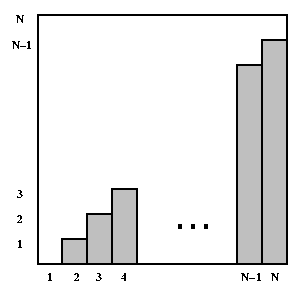
The value of the sum (0+1+2+...+(N-1)) is the sum of the areas of the individual bars. You can see that the bars fill about half of the square. The whole square is an N-by-N square, so its area is N2; therefore, the sum of the areas of the bars is about N2/2. In other words, the time for method createList is proportional to the square of the problem size; if the problem size doubles, the number of operations will quadruple. We say that the worst-case time for createList is quadratic in the problem size.


TEST YOURSELF #2
Consider the following three algorithms for determining whether anyone in the room has the same birthday as you.
Algorithm 1: You say your birthday, and ask whether anyone in the room has the same birthday. If anyone does have the same birthday, they answer yes.
Algorithm 2: You tell the first person your birthday, and ask if they have the same birthday; if they say no, you tell the second person your birthday and ask whether they have the same birthday; etc, for each person in the room.
Algorithm 3: You only ask questions of person 1, who only asks questions of person 2, who only asks questions of person 3, etc. You tell person 1 your birthday, and ask if they have the same birthday; if they say no, you ask them to find out about person 2. Person 1 asks person 2 and tells you the answer. If it is no, you ask person 1 to find out about person 3. Person 1 asks person 2 to find out about person 3, etc.
Question 1: For each algorithm, what is the factor that can affect the number of questions asked (the "problem size")?
Question 2: In the worst case, how many questions will be asked for each of the three algorithms?
Question 3: For each algorithm, say whether it is constant, linear, or quadratic in the problem size in the worst case.

Answer:
Question 1: The problem size is the number of people in the room.
Question 2: Assume there are N people in the room. In algorithm 1 you always ask 1 question. In algorithm 2, the worst case is if no one has your birthday. Here you have to ask every person to figure this out. This is N questions. In algorithm 3, the worst case is the same as algorithm 2. The number of questions is 1 + 2 + 3 + ... + N-1 + N. We showed before that this sum is N(N+1)/2.

Question 3: Given the number of questions you can see that algorithm 1 is constant time, algorithm 2 is linear time, and algorithm 3 is quadratic time in the problem size.

Big-O Notation

We express complexity using big-O notation. For a problem of size N:
  • a constant-time method is "order 1": O(1)
  • a linear-time method is "order N": O(N)
  • a quadratic-time method is "order N squared": O(N2)
Note that the big-O expressions do not have constants or low-order terms. This is because, when N gets large enough, constants and low-order terms don't matter (a constant-time method will be faster than a linear-time method, which will be faster than a quadratic-time method). See below for an example.
Formal definition:
    A function T(N) is O(F(N)) if for some constant c and for all values of N greater than some value n0:
    T(N) <= c * F(N)
The idea is that T(N) is the exact complexity of a method or algorithm as a function of the problem size N, and that F(N) is an upper-bound on that complexity (i.e., the actual time/space or whatever for a problem of size N will be no worse than F(N)). In practice, we want the smallest F(N) -- the least upper bound on the actual complexity.
For example, consider T(N) = 3 * N2 + 5. We can show that T(N) is O(N2) by choosing c = 4 and n0 = 2. This is because for all values of N greater than 2:
3 * N2 + 5 <= 4 * N2
T(N) is not O(N), because whatever constant c and value n0 you choose, I can always find a value of N greater than n0 so that 3 * N2 + 5 is greater than c * N.

How to Determine Complexities

In general, how can you determine the running time of a piece of code? The answer is that it depends on what kinds of statements are used.
  1. Sequence of statements
      statement 1;
      statement 2;
        ...
      statement k;
      
    (Note: this is code that really is exactly k statements; this is not an unrolled loop like the N calls to add shown above.) The total time is found by adding the times for all statements:total time = time(statement 1) + time(statement 2) + ... + time(statement k)
    If each statement is "simple" (only involves basic operations) then the time for each statement is constant and the total time is also constant: O(1). In the following examples, assume the statements are simple unless noted otherwise.
  2. if-then-else statements
      if (condition) {
          sequence of statements 1
      }
      else {
          sequence of statements 2
      }
      
    Here, either sequence 1 will execute, or sequence 2 will execute. Therefore, the worst-case time is the slowest of the two possibilities: max(time(sequence 1), time(sequence 2)). For example, if sequence 1 is O(N) and sequence 2 is O(1) the worst-case time for the whole if-then-else statement would be O(N).
  3. for loops
      for (i = 0; i < N; i++) {
          sequence of statements
      }
      
    The loop executes N times, so the sequence of statements also executes N times. Since we assume the statements are O(1), the total time for the for loop is N * O(1), which is O(N) overall.
  4. Nested loopsFirst we'll consider loops where the number of iterations of the inner loop is independent of the value of the outer loop's index. For example:
      for (i = 0; i < N; i++) {
          for (j = 0; j < M; j++) {
              sequence of statements
          }
      }
      
    The outer loop executes N times. Every time the outer loop executes, the inner loop executes M times. As a result, the statements in the inner loop execute a total of N * M times. Thus, the complexity is O(N * M). In a common special case where the stopping condition of the inner loop is j < N instead of j < M (i.e., the inner loop also executes N times), the total complexity for the two loops is O(N2).Now let's consider nested loops where the number of iterations of the inner loop depends on the value of the outer loop's index. For example:
      for (i = 0; i < N; i++) {
          for (j = i+1; j < N; j++) {
              sequence of statements
          }
      }
      
    Now we can't just multiply the number of iterations of the outer loop times the number of iterations of the inner loop, because the inner loop has a different number of iterations each time. So let's think about how many iterations that inner loop has. That information is given in the following table:
    Value of iNumber of iterations of inner loop
    0N
    1N-1
    2N-2
    ......
    N-22
    N-11
    So we can see that the total number of times the sequence of statements executes is: N + N-1 + N-2 + ... + 3 + 2 + 1. We've seen that formula before: the total is O(N2).

    TEST YOURSELF #3
    What is the worst-case complexity of the each of the following code fragments?
    1. Two loops in a row:
        for (i = 0; i < N; i++) {
            sequence of statements
        }
        for (j = 0; j < M; j++) {
            sequence of statements
        }
        
      How would the complexity change if the second loop went to N instead of M?
    2. A nested loop followed by a non-nested loop:
        for (i = 0; i < N; i++) {
            for (j = 0; j < N; j++) {
                sequence of statements
            }
        }
        for (k = 0; k < N; k++) {
            sequence of statements
        }
        
    3. A nested loop in which the number of times the inner loop executes depends on the value of the outer loop index:
        for (i = 0; i < N; i++) {
            for (j = N; j > i; j--) {
                sequence of statements
            }
        }
        
    Answer:
    1. The first loop is O(N) and the second loop is O(M). Since you don't know which is bigger, you say this is O(N+M). This can also be written as O(max(N,M)). In the case where the second loop goes to N instead of M the complexity is O(N). You can see this from either expression above. O(N+M) becomes O(2N) and when you drop the constant it is O(N). O(max(N,M)) becomes O(max(N,N)) which is O(N).
    2. The first set of nested loops is O(N2) and the second loop is O(N). This is O(max(N2,N)) which is O(N2).
    3. This is very similar to our earlier example of a nested loop where the number of iterations of the inner loop depends on the value of the index of the outer loop. The only difference is that in this example the inner-loop index is counting down from N to i+1. It is still the case that the inner loop executes N times, then N-1, then N-2, etc, so the total number of times the innermost "sequence of statements" execites is O(N2).

  5. Statements with method calls:When a statement involves a method call, the complexity of the statement includes the complexity of the method call. Assume that you know that method f takes constant time, and that method g takes time proportional to (linear in) the value of its parameter k. Then the statements below have the time complexities indicated.
      f(k);  // O(1)
      g(k);  // O(k)
      
    When a loop is involved, the same rule applies. For example:
      for (j = 0; j < N; j++) g(N);
      
    has complexity (N2). The loop executes N times and each method call g(N) is complexity O(N).

    TEST YOURSELF #4
    For each of the following loops with a method call, determine the overall complexity. As above, assume that method f takes constant time, and that method g takes time linear in the value of its parameter.
      1. for (j = 0; j < N; j++) f(j);
      
      2. for (j = 0; j < N; j++) g(j);
      
      3. for (j = 0; j < N; j++) g(k);
      
    Answer: 

  1. Each call to f(j) is O(1). The loop executes N times so it is N x O(1) or O(N).
  2. The first time the loop executes j is 0 and g(0) takes "no operations". The next time j is 1 and g(1) takes 1 operations. The last time the loop executes j is N-1 and g(N-1) takes N-1 operations. The total work is the sum of the first N-1 numbers and is O(N2).
  3. Each time through the loop g(k) takes k operations and the loop executes N times. Since you don't know the relative size of k and N, the overall complexity is O(N x k).

Best-case and Average-case Complexity

Some methods may require different amounts of time on different calls, even when the problem size is the same for both calls. For example, consider the add method that adds an item to the end of the list. In the worst case (the array is full), that method requires time proportional to the number of items in the list (because it has to copy all of them into the new, larger array). However, when the array is not full, add will only have to copy one value into the array, so in that case its time is independent of the length of the list; i.e., constant time.
In general, we may want to consider the best and average time requirements of a method as well as its worst-case time requirements. Which is considered the most important will depend on several factors. For example, if a method is part of a time-critical system like one that controls an airplane, the worst-case times are probably the most important (if the plane is flying towards a mountain and the controlling program can't make the next course correction until it has performed a computation, then the best-case and average-case times for that computation are not relevant -- the computation needs to be guaranteed to be fast enough to finish before the plane hits the mountain).
On the other hand, if occasionally waiting a long time for an answer is merely inconvenient (as opposed to life-threatening), it may be better to use an algorithm with a slow worst-case time and a fast average-case time, rather than one with so-so times in both the average and worst cases.
Note that calculating the average-case time for a method can be tricky. You need to consider all possible values for the important factors, and whether they will be distributed evenly.

When do Constants Matter?

Recall that when we use big-O notation, we drop constants and low-order terms. This is because when the problem size gets sufficiently large, those terms don't matter. However, this means that two algorithms can have thesame big-O time complexity, even though one is always faster than the other. For example, suppose algorithm 1 requires N2 time, and algorithm 2 requires 10 * N2 + N time. For both algorithms, the time is O(N2), but algorithm 1 will always be faster than algorithm 2. In this case, the constants and low-order terms do matter in terms of which algorithm is actually faster.
However, it is important to note that constants do not matter in terms of the question of how an algorithm "scales" (i.e., how does the algorithm's time change when the problem size doubles). Although an algorithm that requires N2 time will always be faster than an algorithm that requires 10*N2 time, for both algorithms, if the problem size doubles, the actual time will quadruple.
When two algorithms have different big-O time complexity, the constants and low-order terms only matter when the problem size is small. For example, even if there are large constants involved, a linear-time algorithm will always eventually be faster than a quadratic-time algorithm. This is illustrated in the following table, which shows the value of 100*N (a time that is linear in N) and the value of N2/100 (a time that is quadratic in N) for some values of N. For values of N less than 104, the quadratic time is smaller than the linear time. However, for all values of N greater than 104, the linear time is smaller.
N100*NN2/100
102104102
103105104
104106106
105107108
1061081010
1071091012

Saturday, April 22, 2023

Error Recovery


Terminology

  • system consists of a set of hardware and software components and is designed to provide a specified service.
  • Failure of a system occurs when the system does not perform its services in the manner specified.
  • An erroneous state of the system is a state which could lead to a system failure by a sequence of valid state transitions
  • fault is an anomalous physical condition.
  • An error is a manifestation of a fault in a system, which can lead to system failure.

Recovery

  • Failure recovery is a process that restores an erroneous state to an error-free state. (after a failure, restoring system to its "normal" state)

Failure Classification

  • process failure
  • system failure
  • secondary storage failure
  • communication medium failure
What are some causes for each?

Tolerating Process Failures

  • signal process to recover internally
  • restart process from a prior state
  • abort process
What are some situations where each is appropriate?

Recovering from System Failures

  • amnesia -- restart in predefined state
  • partial amnesia -- reset part of the state to predefined
  • pause -- roll back to before failure
  • halting -- give up

Tolerating Secondary Storage Failures

  • archiving (periodic backup)
  • mirroring (continuous)
  • activity logging

Tolerating Communication Medium Failures

  • ack & resend
  • more complex fault-tolerant algorithms

Backward versus Forward Error Recovery

  • skip forward to a new correct state
    • requires contextual knowledge of what "forward" is
  • go back to a previous correct state
    • overhead: takes time to save and restore state
    • fault may repeat (¥ cycling)
    • recovery may be impossible

Backward Error Recovery

  • based on recovery points
  • two approaches:
    1. operation-based recovery
    2. state-based recovery

System Model

Stable Storage

  • does not lose information in the event of system failure
  • is used to keep logs & recovery points
  • algorithms in this chapter assume an underlying stable storage system already exists

Two Approaches to Fault Tolerance

  • operation based
    • record a log (audit trail) of the operations performed
    • restore previous state by reversing steps
  • state based
    • record a snapshot of the state (checkpoint)
    • restore state by reloading snapshot (rollback)
Practical systems employ a combination of the two approaches, e.g., logging with periodic full-DB snapshots for archive.

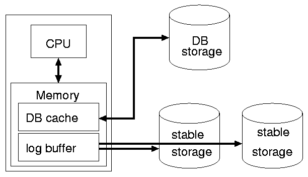
Fundamental Issues in Crash Recovery

  • disk writes are only atomic by sector
  • updates and commits require multiple writes
  • a crash may occur between writes
  • log contains record of updates, commits, and aborts
  • data is written to disk asynchronously
    • DB is cached
    • log is buffered
The textbook jumps right into the problem of supporting crash recovery, without first reviewing any basic transaction models. The following are two more basic models than those mentioned in the text.

Basic Deferred-Update Model

  • save a transaction's updates as it runs, in temporary storage
  • use the saved updates to update the database when the transaction commits
  • update: record a redo record (e.g. the new value of the item being updated) in an intention list
  • read: combine the intention list and the database to determine the desired value
  • commit: update the database by applying the intention list in order, starting with the first operation done by the transaction
  • abort: discard the transaction's intention list

Basic Update-In-Place Model

  • update the DB as transaction runs
  • undo the updates if the transaction aborts
  • update: record an undo record (e.g., the old value of the item being updated) to an undo log, and then update the database
  • read:
  • commit: discard the transaction's undo log
  • abort: use the undo records in the transaction's undo log to back out the transaction's updates, by backing out the operations in the reverse of the order in which they were originally done
What provides for disk crash recovery?

Extended Update-In-Place Model

  • update: modify the online DB and record both undo and redo records, including:
    • name/location of object
    • old state/value of object (for undo)
    • new state/value of object (for redo)
    in a safe order
  • read: read the current value and apply the transaction's undo log
  • commit: discard/invalidate the transaction's undo log
  • abort: use the undo records in the transaction's undo log to back out the transaction's updates
Where does the stable storage fit in?

Crash Recovery with Update-In-Place

We now have a way to reconstruct the DB system in event of a crash, starting from an archived snapshot and the subsequent log:
  • transactions not logged as committed are treated as aborted
  • back out active or aborted transactions, using undo records
  • do DB updates that may have been in cache, using redo records
If we are starting with a snapshot, why do we need to worry about active, uncommitted, and aborted transactions?

Problem: DB write before log write

There is a defect in the above scheme
  • if the cached new value of X is written to DB on disk
  • and then the system crashes, before the old value of X is written to log
How to solve?

Solution: Write-Ahead-Log

Before a block is written to DB disk, make sure the corresponding undo record is completely written to the log disk.
The log must be forced to disk as part of committing a transaction.

Crash Recovery with Write-Ahead-Log

  • redo phase: redo all the updates in the log, including undo operations of aborted transactions
  • undo phase: abort all transactions that have no commit or abort record in the log, using the usual undo records in the log

State Based Approach

  • based on checkpoints of entire state of process
  • recovery does rollback to checkpointed state
  • use of shadow pages can reduce size of checkpoints

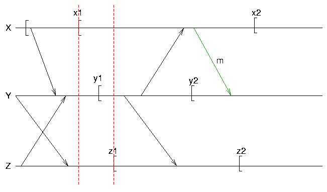
Problems in Distributed/Concurrent Systems

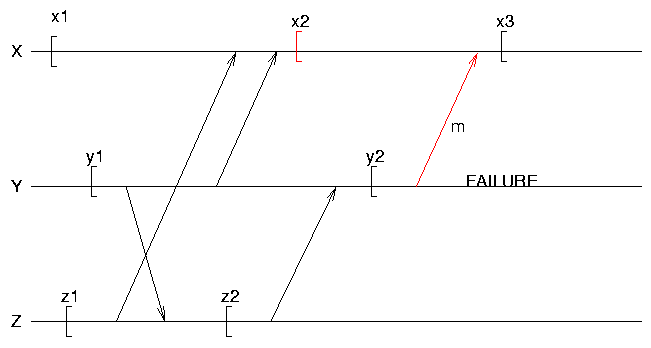
  • communicating processes must coordinate checkpoints & rollbacks
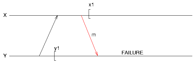
  • lost messages
  • orphan messages
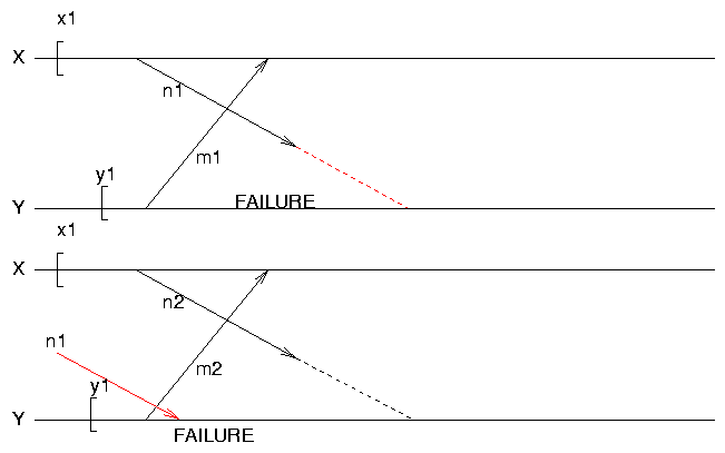
  • livelocks

Orphan Messages

Note domino effect if Z is rolled back

Lost Messages

What is the difference between a lost message and an orphan message?

Livelock

These all motivate need for coordinating checkpoints & recovery

Strongly Consistent Set of Checkpoints

There is no information flow between any processes in the set during the time interval spanned by the checkpoints, i.e., no messages in transit.

Consistent Set of Checkpoints

There may be information flow between the processes, but each message recorded as received should be recorded as sent. That is, there are no orphan messages.
What is the remaining problem here?

Tuesday, October 4, 2022

Operating-System Structures

Operating-System Services


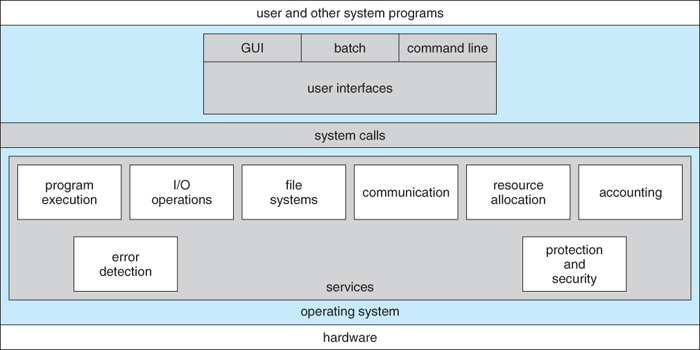
Figure 2.1 - A view of operating system services
OSes provide environments in which programs run, and services for the users of the system, including:
  • User Interfaces - Means by which users can issue commands to the system. Depending on the system these may be a command-line interface ( e.g. sh, csh, ksh, tcsh, etc. ), a GUI interface ( e.g. Windows, X-Windows, KDE, Gnome, etc. ), or a batch command systems. The latter are generally older systems using punch cards of job-control language, JCL, but may still be used today for specialty systems designed for a single purpose.
  • Program Execution - The OS must be able to load a program into RAM, run the program, and terminate the program, either normally or abnormally.
  • I/O Operations - The OS is responsible for transferring data to and from I/O devices, including keyboards, terminals, printers, and storage devices.
  • File-System Manipulation - In addition to raw data storage, the OS is also responsible for maintaining directory and subdirectory structures, mapping file names to specific blocks of data storage, and providing tools for navigating and utilizing the file system.
  • Communications - Inter-process communications, IPC, either between processes running on the same processor, or between processes running on separate processors or separate machines. May be implemented as either shared memory or message passing, ( or some systems may offer both. )
  • Error Detection - Both hardware and software errors must be detected and handled appropriately, with a minimum of harmful repercussions. Some systems may include complex error avoidance or recovery systems, including backups, RAID drives, and other redundant systems. Debugging and diagnostic tools aid users and administrators in tracing down the cause of problems.
Other systems aid in the efficient operation of the OS itself:
  • Resource Allocation - E.g. CPU cycles, main memory, storage space, and peripheral devices. Some resources are managed with generic systems and others with very carefully designed and specially tuned systems, customized for a particular resource and operating environment.
  • Accounting - Keeping track of system activity and resource usage, either for billing purposes or for statistical record keeping that can be used to optimize future performance.
  • Protection and Security - Preventing harm to the system and to resources, either through wayward internal processes or malicious outsiders. Authentication, ownership, and restricted access are obvious parts of this system. Highly secure systems may log all process activity down to excruciating detail, and security regulation dictate the storage of those records on permanent non-erasable medium for extended times in secure ( off-site ) facilities.

2.2 User Operating-System Interface

2.2.1 Command Interpreter

  • Gets and processes the next user request, and launches the requested programs.
  • In some systems the CI may be incorporated directly into the kernel.
  • More commonly the CI is a separate program that launches once the user logs in or otherwise accesses the system.
  • UNIX, for example, provides the user with a choice of different shells, which may either be configured to launch automatically at login, or which may be changed on the fly. ( Each of these shells uses a different configuration file of initial settings and commands that are executed upon startup. )
  • Different shells provide different functionality, in terms of certain commands that are implemented directly by the shell without launching any external programs. Most provide at least a rudimentary command interpretation structure for use in shell script programming ( loops, decision constructs, variables, etc. )
  • An interesting distinction is the processing of wild card file naming and I/O re-direction. On UNIX systems those details are handled by the shell, and the program which is launched sees only a list of filenames generated by the shell from the wild cards. On a DOS system, the wild cards are passed along to the programs, which can interpret the wild cards as the program sees fit.

Figure 2.2 - The Bourne shell command interpreter in Solaris 10

2.2.2 Graphical User Interface, GUI

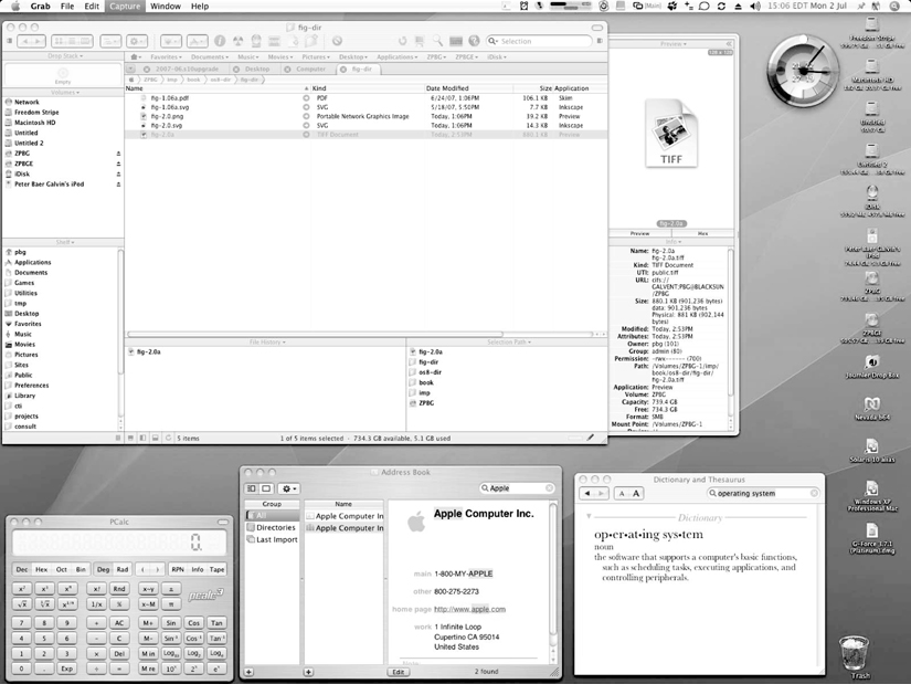
  • Generally implemented as a desktop metaphor, with file folders, trash cans, and resource icons.
  • Icons represent some item on the system, and respond accordingly when the icon is activated.
  • First developed in the early 1970's at Xerox PARC research facility.
  • In some systems the GUI is just a front end for activating a traditional command line interpreter running in the background. In others the GUI is a true graphical shell in its own right.
  • Mac has traditionally provided ONLY the GUI interface. With the advent of OSX ( based partially on UNIX ), a command line interface has also become available.
  • Because mice and keyboards are impractical for small mobile devices, these normally use a touch-screen interface today, that responds to various patterns of swipes or "gestures". When these first came out they often had a physical keyboard and/or a trackball of some kind built in, but today a virtual keyboard is more commonly implemented on the touch screen.

Figure 2.3 - The iPad touchscreen

2.2.3 Choice of interface

  • Most modern systems allow individual users to select their desired interface, and to customize its operation, as well as the ability to switch between different interfaces as needed. System administrators generally determine which interface a user starts with when they first log in.
  • GUI interfaces usually provide an option for a terminal emulator window for entering command-line commands.
  • Command-line commands can also be entered into shell scripts, which can then be run like any other programs.

Figure 2.4 - The Mac OS X GUI

2.3 System Calls

  • System calls provide a means for user or application programs to call upon the services of the operating system.
  • Generally written in C or C++, although some are written in assembly for optimal performance.
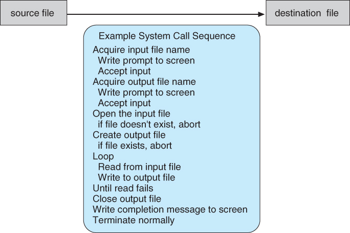
  • Figure 2.4 illustrates the sequence of system calls required to copy a file:

Figure 2.5 - Example of how system calls are used.
  • You can use "strace" to see more examples of the large number of system calls invoked by a single simple command. Read the man page for strace, and try some simple examples. ( strace mkdir temp, strace cd temp, strace date > t.t, strace cp t.t t.2, etc. )
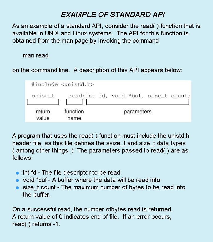
  • Most programmers do not use the low-level system calls directly, but instead use an "Application Programming Interface", API. The following sidebar shows the read( ) call available in the API on UNIX based systems::

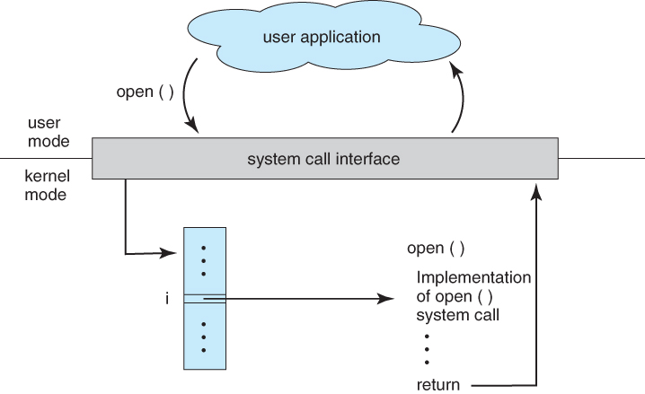
The use of APIs instead of direct system calls provides for greater program portability between different systems. The API then makes the appropriate system calls through the system call interface, using a table lookup to access specific numbered system calls, as shown in Figure 2.6:

Figure 2.6 - The handling of a user application invoking the open( ) system call
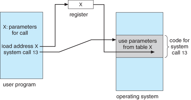
  • Parameters are generally passed to system calls via registers, or less commonly, by values pushed onto the stack. Large blocks of data are generally accessed indirectly, through a memory address passed in a register or on the stack, as shown in Figure 2.7:

Figure 2.7 - Passing of parameters as a table

2.4 Types of System Calls

Six major categories, as outlined in Figure 2.8 and the following six subsections:

( Sixth type, protection, not shown here but described below. )
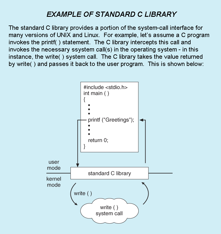
  • Standard library calls may also generate system calls, as shown here:


2.4.1 Process Control

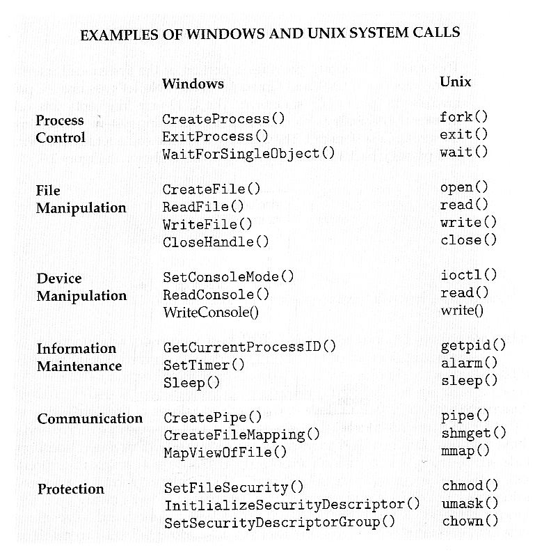
  • Process control system calls include end, abort, load, execute, create process, terminate process, get/set process attributes, wait for time or event, signal event, and allocate and free memory.
  • Processes must be created, launched, monitored, paused, resumed,and eventually stopped.
  • When one process pauses or stops, then another must be launched or resumed
  • When processes stop abnormally it may be necessary to provide core dumps and/or other diagnostic or recovery tools.
  • Compare DOS ( a single-tasking system ) with UNIX ( a multi-tasking system ).
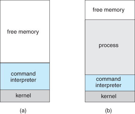
    • When a process is launched in DOS, the command interpreter first unloads as much of itself as it can to free up memory, then loads the process and transfers control to it. The interpreter does not resume until the process has completed, as shown in Figure 2.9:

Figure 2.9 - MS-DOS execution. (a) At system startup. (b) Running a program.
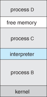
    • Because UNIX is a multi-tasking system, the command interpreter remains completely resident when executing a process, as shown in Figure 2.11 below.
      • The user can switch back to the command interpreter at any time, and can place the running process in the background even if it was not originally launched as a background process.
      • In order to do this, the command interpreter first executes a "fork" system call, which creates a second process which is an exact duplicate ( clone ) of the original command interpreter. The original process is known as the parent, and the cloned process is known as the child, with its own unique process ID and parent ID.
      • The child process then executes an "exec" system call, which replaces its code with that of the desired process.
      • The parent ( command interpreter ) normally waits for the child to complete before issuing a new command prompt, but in some cases it can also issue a new prompt right away, without waiting for the child process to complete. ( The child is then said to be running "in the background", or "as a background process". )

Figure 2.10 - FreeBSD running multiple programs

2.4.2 File Management

  • File management system calls include create file, delete file, open, close, read, write, reposition, get file attributes, and set file attributes.
  • These operations may also be supported for directories as well as ordinary files.
  • ( The actual directory structure may be implemented using ordinary files on the file system, or through other means. Further details will be covered in chapters 11 and 12. )

2.4.3 Device Management

  • Device management system calls include request device, release device, read, write, reposition, get/set device attributes, and logically attach or detach devices.
  • Devices may be physical ( e.g. disk drives ), or virtual / abstract ( e.g. files, partitions, and RAM disks ).
  • Some systems represent devices as special files in the file system, so that accessing the "file" calls upon the appropriate device drivers in the OS. See for example the /dev directory on any UNIX system.

2.4.4 Information Maintenance

  • Information maintenance system calls include calls to get/set the time, date, system data, and process, file, or device attributes.
  • Systems may also provide the ability to dump memory at any time, single step programs pausing execution after each instruction, and tracing the operation of programs, all of which can help to debug programs.

2.4.5 Communication

  • Communication system calls create/delete communication connection, send/receive messages, transfer status information, and attach/detach remote devices.
  • The message passing model must support calls to:
    • Identify a remote process and/or host with which to communicate.
    • Establish a connection between the two processes.
    • Open and close the connection as needed.
    • Transmit messages along the connection.
    • Wait for incoming messages, in either a blocking or non-blocking state.
    • Delete the connection when no longer needed.
  • The shared memory model must support calls to:
    • Create and access memory that is shared amongst processes ( and threads. )
    • Provide locking mechanisms restricting simultaneous access.
    • Free up shared memory and/or dynamically allocate it as needed.
  • Message passing is simpler and easier, ( particularly for inter-computer communications ), and is generally appropriate for small amounts of data.
  • Shared memory is faster, and is generally the better approach where large amounts of data are to be shared, ( particularly when most processes are reading the data rather than writing it, or at least when only one or a small number of processes need to change any given data item. )

2.4.6 Protection

  • Protection provides mechanisms for controlling which users / processes have access to which system resources.
  • System calls allow the access mechanisms to be adjusted as needed, and for non-priveleged users to be granted elevated access permissions under carefully controlled temporary circumstances.
  • Once only of concern on multi-user systems, protection is now important on all systems, in the age of ubiquitous network connectivity.

2.5 System Programs

  • System programs provide OS functionality through separate applications, which are not part of the kernel or command interpreters. They are also known as system utilities or system applications.
  • Most systems also ship with useful applications such as calculators and simple editors, ( e.g. Notepad ). Some debate arises as to the border between system and non-system applications.
  • System programs may be divided into these categories:
    • File management - programs to create, delete, copy, rename, print, list, and generally manipulate files and directories.
    • Status information - Utilities to check on the date, time, number of users, processes running, data logging, etc. System registries are used to store and recall configuration information for particular applications.
    • File modification - e.g. text editors and other tools which can change file contents.
    • Programming-language support - E.g. Compilers, linkers, debuggers, profilers, assemblers, library archive management, interpreters for common languages, and support for make.
    • Program loading and execution - loaders, dynamic loaders, overlay loaders, etc., as well as interactive debuggers.
    • Communications - Programs for providing connectivity between processes and users, including mail, web browsers, remote logins, file transfers, and remote command execution.
    • Background services - System daemons are commonly started when the system is booted, and run for as long as the system is running, handling necessary services. Examples include network daemons, print servers, process schedulers, and system error monitoring services.
  • Most operating systems today also come complete with a set of application programs to provide additional services, such as copying files or checking the time and date.
  • Most users' views of the system is determined by their command interpreter and the application programs. Most never make system calls, even through the API, ( with the exception of simple ( file ) I/O in user-written programs. )

2.6 Operating-System Design and Implementation

2.6.1 Design Goals

  • Requirements define properties which the finished system must have, and are a necessary first step in designing any large complex system.
    • User requirements are features that users care about and understand, and are written in commonly understood vernacular. They generally do not include any implementation details, and are written similar to the product description one might find on a sales brochure or the outside of a shrink-wrapped box.
    • System requirements are written for the developers, and include more details about implementation specifics, performance requirements, compatibility constraints, standards compliance, etc. These requirements serve as a "contract" between the customer and the developers, ( and between developers and subcontractors ), and can get quite detailed.
  • Requirements for operating systems can vary greatly depending on the planned scope and usage of the system. ( Single user / multi-user, specialized system / general purpose, high/low security, performance needs, operating environment, etc. )

2.6.2 Mechanisms and Policies

  • Policies determine what is to be done. Mechanisms determine how it is to be implemented.
  • If properly separated and implemented, policy changes can be easily adjusted without re-writing the code, just by adjusting parameters or possibly loading new data / configuration files. For example the relative priority of background versus foreground tasks.

2.6.3 Implementation

  • Traditionally OSes were written in assembly language. This provided direct control over hardware-related issues, but inextricably tied a particular OS to a particular HW platform.
  • Recent advances in compiler efficiencies mean that most modern OSes are written in C, or more recently, C++. Critical sections of code are still written in assembly language, ( or written in C, compiled to assembly, and then fine-tuned and optimized by hand from there. )
  • Operating systems may be developed using emulators of the target hardware, particularly if the real hardware is unavailable ( e.g. not built yet ), or not a suitable platform for development, ( e.g. smart phones, game consoles, or other similar devices. )

2.7 Operating-System Structure

For efficient performance and implementation an OS should be partitioned into separate subsystems, each with carefully defined tasks, inputs, outputs, and performance characteristics. These subsystems can then be arranged in various architectural configurations:

2.7.1 Simple Structure

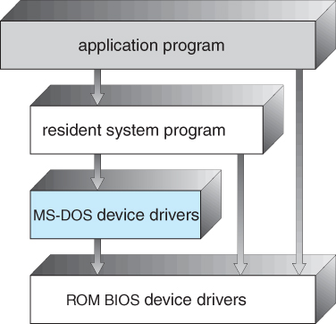
When DOS was originally written its developers had no idea how big and important it would eventually become. It was written by a few programmers in a relatively short amount of time, without the benefit of modern software engineering techniques, and then gradually grew over time to exceed its original expectations. It does not break the system into subsystems, and has no distinction between user and kernel modes, allowing all programs direct access to the underlying hardware. ( Note that user versus kernel mode was not supported by the 8088 chip set anyway, so that really wasn't an option back then. )

Figure 2.11 - MS-DOS layer structure
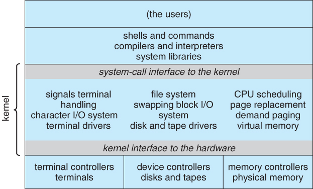
The original UNIX OS used a simple layered approach, but almost all the OS was in one big layer, not really breaking the OS down into layered subsystems:


Figure 2.12 - Traditional UNIX system structure

2.7.2 Layered Approach

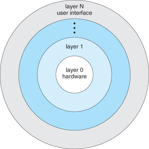
  • Another approach is to break the OS into a number of smaller layers, each of which rests on the layer below it, and relies solely on the services provided by the next lower layer.
  • This approach allows each layer to be developed and debugged independently, with the assumption that all lower layers have already been debugged and are trusted to deliver proper services.
  • The problem is deciding what order in which to place the layers, as no layer can call upon the services of any higher layer, and so many chicken-and-egg situations may arise.
  • Layered approaches can also be less efficient, as a request for service from a higher layer has to filter through all lower layers before it reaches the HW, possibly with significant processing at each step.

Figure 2.13 - A layered operating system

2.7.3 Microkernels

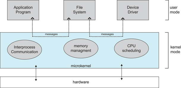
  • The basic idea behind micro kernels is to remove all non-essential services from the kernel, and implement them as system applications instead, thereby making the kernel as small and efficient as possible.
  • Most microkernels provide basic process and memory management, and message passing between other services, and not much more.
  • Security and protection can be enhanced, as most services are performed in user mode, not kernel mode.
  • System expansion can also be easier, because it only involves adding more system applications, not rebuilding a new kernel.
  • Mach was the first and most widely known microkernel, and now forms a major component of Mac OSX.
  • Windows NT was originally microkernel, but suffered from performance problems relative to Windows 95. NT 4.0 improved performance by moving more services into the kernel, and now XP is back to being more monolithic.
  • Another microkernel example is QNX, a real-time OS for embedded systems.

Figure 2.14 - Architecture of a typical microkernel

2.7.4 Modules

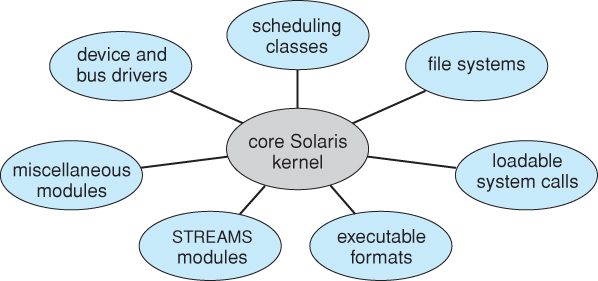
  • Modern OS development is object-oriented, with a relatively small core kernel and a set of modules which can be linked in dynamically. See for example the Solaris structure, as shown in Figure 2.13 below.
  • Modules are similar to layers in that each subsystem has clearly defined tasks and interfaces, but any module is free to contact any other module, eliminating the problems of going through multiple intermediary layers, as well as the chicken-and-egg problems.
  • The kernel is relatively small in this architecture, similar to microkernels, but the kernel does not have to implement message passing since modules are free to contact each other directly.

Figure 2.15 - Solaris loadable modules

2.7.5 Hybrid Systems

  • Most OSes today do not strictly adhere to one architecture, but are hybrids of several.

2.7.5.1 Mac OS X

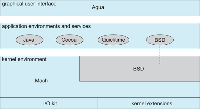
  • The Max OSX architecture relies on the Mach microkernel for basic system management services, and the BSD kernel for additional services. Application services and dynamically loadable modules ( kernel extensions ) provide the rest of the OS functionality:

Figure 2.16 - The Mac OS X structure

2.7.5.2 iOS

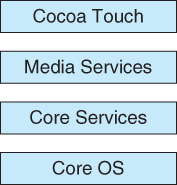
  • The iOS operating system was developed by Apple for iPhones and iPads. It runs with less memory and computing power needs than Max OS X, and supports touchscreen interface and graphics for small screens:

Figure 2.17 - Architecture of Apple's iOS.

2.7.5.3 Android

  • The Android OS was developed for Android smartphones and tablets by the Open Handset Alliance, primarily Google.
  • Android is an open-source OS, as opposed to iOS, which has lead to its popularity.
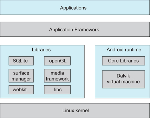
  • Android includes versions of Linux and a Java virtual machine both optimized for small platforms.
  • Android apps are developed using a special Java-for-Android development environment.

Figure 2.18 - Architecture of Google's Android

2.8 Operating-System Debugging

Kernighan's Law
"Debugging is twice as hard as writing the code in the first place. Therefore,
if you write the code as cleverly as possible, you are, by definition, not smart
enough to debug it."
  • Debugging here includes both error discovery and elimination and performance tuning.

2.8.1 Failure Analysis

  • Debuggers allow processes to be executed stepwise, and provide for the examination of variables and expressions as the execution progresses.
  • Profilers can document program execution, to produce statistics on how much time was spent on different sections or even lines of code.
  • If an ordinary process crashes, a memory dump of the state of that process's memory at the time of the crash can be saved to a disk file for later analysis.
    • The program must be specially compiled to include debugging information, which may slow down its performance.
  • These approaches don't really work well for OS code, for several reasons:
    • The performance hit caused by adding the debugging ( tracing ) code would be unacceptable. ( Particularly if one tried to "single-step" the OS while people were trying to use it to get work done! )
    • Many parts of the OS run in kernel mode, and make direct access to the hardware.
    • If an error occurred during one of the kernel's file-access or direct disk-access routines, for example, then it would not be practical to try to write a crash dump into an ordinary file on the filesystem.
      • Instead the kernel crash dump might be saved to a special unallocated portion of the disk reserved for that purpose.

2.8.2 Performance Tuning

  • Performance tuning ( debottlenecking ) requires monitoring system performance.
  • One approach is for the system to record important events into log files, which can then be analyzed by other tools. These traces can also be used to evaluate how a proposed new system would perform under the same workload.
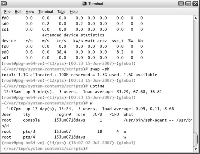
  • Another approach is to provide utilities that will report system status upon demand, such as the unix "top" command. ( w, uptime, ps, etc. )
  • System utilities may provide monitoring support.

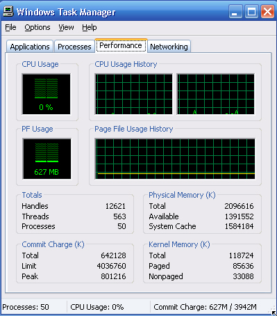
Figure 2.19 - The Windows task manager.

2.8.3 DTrace

  • DTrace is a special facility for tracing a running OS, developed for Solaris 10.
  • DTrace adds "probes" directly into the OS code, which can be queried by "probe consumers".
  • Probes are removed when not in use, so the DTrace facility has zero impact on the system when not being used, and a proportional impact in use.
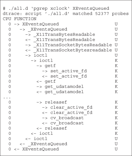
  • Consider, for example, the trace of an ioctl system call as shown in Figure 2.22 below.

Figure 2.20 - Solaris 10 dtrace follows a system call within the kernel
  • Probe code is restricted to be "safe", ( e.g. no loops allowed ), and to use a minimum of system resources.
  • When a probe fires, enabling control blocks, ECBs, are performed, each having the structure of an if-then block
  • When a consumer terminates, the ECBs associated with that consumer are removed. When no more ECBs remain interested in a particular probe, then that probe is also removed.
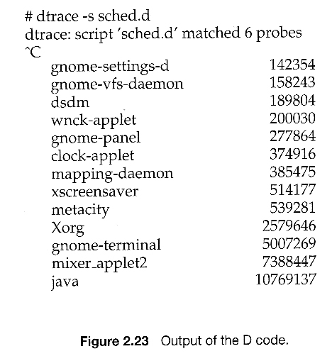
  • For example, the following D code monitors the CPU time of each process running with user ID of 101. The output is shown in Figure 2.23 below.
    sched:::on-cpu
    uid == 101
    {
         self->ts = timestamp;
    }
    sched:::off-cpu
    self->ts
    {
         @time[execname] = sum( timestamp - self->ts );
         self->ts = 0;
    }

    Figure 2.21
  • Use of DTrace is restricted, due to the direct access to ( and ability to change ) critical kernel data structures.
  • Because DTrace is open-source, it is being adopted by several UNIX distributions. Others are busy producing similar utilities.

2.9 Operating-System Generation

  • OSes may be designed and built for a specific HW configuration at a specific site, but more commonly they are designed with a number of variable parameters and components, which are then configured for a particular operating environment.
  • Systems sometimes need to be re-configured after the initial installation, to add additional resources, capabilities, or to tune performance, logging, or security.
  • Information that is needed to configure an OS include:
    • What CPU(s) are installed on the system, and what optional characteristics does each have?
    • How much RAM is installed? ( This may be determined automatically, either at install or boot time. )
    • What devices are present? The OS needs to determine which device drivers to include, as well as some device-specific characteristics and parameters.
    • What OS options are desired, and what values to set for particular OS parameters. The latter may include the size of the open file table, the number of buffers to use, process scheduling ( priority ) parameters, disk scheduling algorithms, number of slots in the process table, etc.
  • At one extreme the OS source code can be edited, re-compiled, and linked into a new kernel.
  • More commonly configuration tables determine which modules to link into the new kernel, and what values to set for some key important parameters. This approach may require the configuration of complicated makefiles, which can be done either automatically or through interactive configuration programs; Then make is used to actually generate the new kernel specified by the new parameters.
  • At the other extreme a system configuration may be entirely defined by table data, in which case the "rebuilding" of the system merely requires editing data tables.
  • Once a system has been regenerated, it is usually required to reboot the system to activate the new kernel. Because there are possibilities for errors, most systems provide some mechanism for booting to older or alternate kernels.

2.10 System Boot

The general approach when most computers boot up goes something like this:
  • When the system powers up, an interrupt is generated which loads a memory address into the program counter, and the system begins executing instructions found at that address. This address points to the "bootstrap" program located in ROM chips ( or EPROM chips ) on the motherboard.
  • The ROM bootstrap program first runs hardware checks, determining what physical resources are present and doing power-on self tests ( POST ) of all HW for which this is applicable. Some devices, such as controller cards may have their own on-board diagnostics, which are called by the ROM bootstrap program.
  • The user generally has the option of pressing a special key during the POST process, which will launch the ROM BIOS configuration utility if pressed. This utility allows the user to specify and configure certain hardware parameters as where to look for an OS and whether or not to restrict access to the utility with a password.
    • Some hardware may also provide access to additional configuration setup programs, such as for a RAID disk controller or some special graphics or networking cards.
  • Assuming the utility has not been invoked, the bootstrap program then looks for a non-volatile storage device containing an OS. Depending on configuration, it may look for a floppy drive, CD ROM drive, or primary or secondary hard drives, in the order specified by the HW configuration utility.
  • Assuming it goes to a hard drive, it will find the first sector on the hard drive and load up the fdisk table, which contains information about how the physical hard drive is divided up into logical partitions, where each partition starts and ends, and which partition is the "active" partition used for booting the system.
  • There is also a very small amount of system code in the portion of the first disk block not occupied by the fdisk table. This bootstrap code is the first step that is not built into the hardware, i.e. the first part which might be in any way OS-specific. Generally this code knows just enough to access the hard drive, and to load and execute a ( slightly ) larger boot program.
  • For a single-boot system, the boot program loaded off of the hard disk will then proceed to locate the kernel on the hard drive, load the kernel into memory, and then transfer control over to the kernel. There may be some opportunity to specify a particular kernel to be loaded at this stage, which may be useful if a new kernel has just been generated and doesn't work, or if the system has multiple kernels available with different configurations for different purposes. ( Some systems may boot different configurations automatically, depending on what hardware has been found in earlier steps. )
  • For dual-boot or multiple-boot systems, the boot program will give the user an opportunity to specify a particular OS to load, with a default choice if the user does not pick a particular OS within a given time frame. The boot program then finds the boot loader for the chosen single-boot OS, and runs that program as described in the previous bullet point.
  • Once the kernel is running, it may give the user the opportunity to enter into single-user mode, also known as maintenance mode. This mode launches very few if any system services, and does not enable any logins other than the primary log in on the console. This mode is used primarily for system maintenance and diagnostics.
  • When the system enters full multi-user multi-tasking mode, it examines configuration files to determine which system services are to be started, and launches each of them in turn. It then spawns login programs ( gettys ) on each of the login devices which have been configured to enable user logins.
    • ( The getty program initializes terminal I/O, issues the login prompt, accepts login names and passwords, and authenticates the user. If the user's password is authenticated, then the getty looks in system files to determine what shell is assigned to the user, and then "execs" ( becomes ) the user's shell. The shell program will look in system and user configuration files to initialize itself, and then issue prompts for user commands. Whenever the shell dies, either through logout or other means, then the system will issue a new getty for that terminal device. )

2.11 Summary


Old 2.8 Virtual Machines ( Moved elsewhere in the 9th edition. )

  • The concept of a virtual machine is to provide an interface that looks like independent hardware, to multiple different OSes running simultaneously on the same physical hardware. Each OS believes that it has access to and control over its own CPU, RAM, I/O devices, hard drives, etc.
  • One obvious use for this system is for the development and testing of software that must run on multiple platforms and/or OSes.
  • One obvious difficulty involves the sharing of hard drives, which are generally partitioned into separate smaller virtual disks for each operating OS.

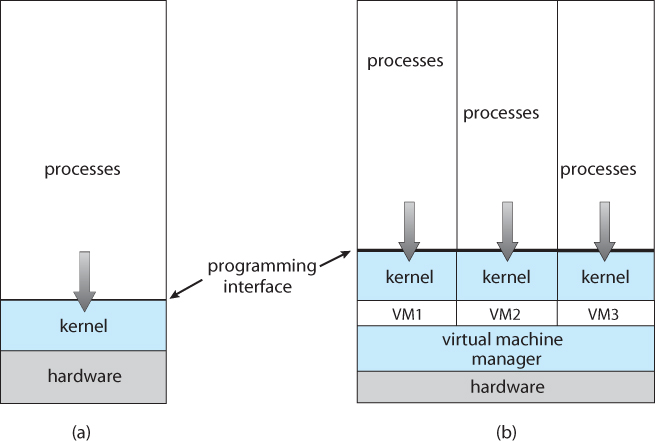
Figure 16.1 - System models. (a) Nonvirtual machine. (b)Virtual machine.

2.8.1 History

  • Virtual machines first appeared as the VM Operating System for IBM mainframes in 1972.

2.8.2 Benefits

  • Each OS runs independently of all the others, offering protection and security benefits.
  • ( Sharing of physical resources is not commonly implemented, but may be done as if the virtual machines were networked together. )
  • Virtual machines are a very useful tool for OS development, as they allow a user full access to and control over a virtual machine, without affecting other users operating the real machine.
  • As mentioned before, this approach can also be useful for product development and testing of SW that must run on multiple OSes / HW platforms.

2.8.3 Simulation

  • An alternative to creating an entire virtual machine is to simply run an emulator, which allows a program written for one OS to run on a different OS.
  • For example, a UNIX machine may run a DOS emulator in order to run DOS programs, or vice-versa.
  • Emulators tend to run considerably slower than the native OS, and are also generally less than perfect.

2.8.4 Para-virtualization

  • Para-virtualization is another variation on the theme, in which an environment is provided for the guest program that is similar to its native OS, without trying to completely mimic it.
  • Guest programs must also be modified to run on the para-virtual OS.
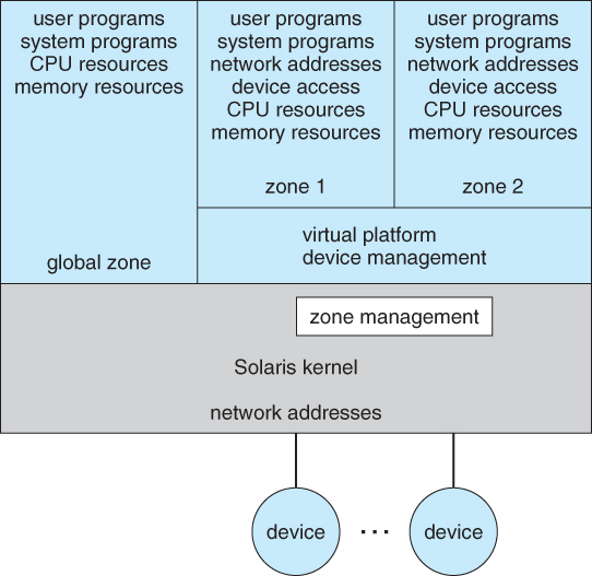
  • Solaris 10 uses a zone system, in which the low-level hardware is not virtualized, but the OS and its devices ( device drivers ) are.
    • Within a zone, processes have the view of an isolated system, in which only the processes and resources within that zone are seen to exist.
    • Figure 2.18 shows a Solaris system with the normal "global" operating space as well as two additional zones running on a small virtualization layer.

Figure 16.7 - Solaris 10 with two zones.

2.8.5 Implementation

  • Implementation may be challenging, partially due to the consequences of user versus kernel mode.
    • Each of the simultaneously running kernels needs to operate in kernel mode at some point, but the virtual machine actually runs in user mode.
    • So the kernel mode has to be simulated for each of the loaded OSes, and kernel system calls passed through the virtual machine into a true kernel mode for eventual HW access.
  • The virtual machines may run slower, due to the increased levels of code between applications and the HW, or they may run faster, due to the benefits of caching. ( And virtual devices may also be faster than real devices, such as RAM disks which are faster than physical disks. )

2.8.6 Examples

2.8.6.1 VMware
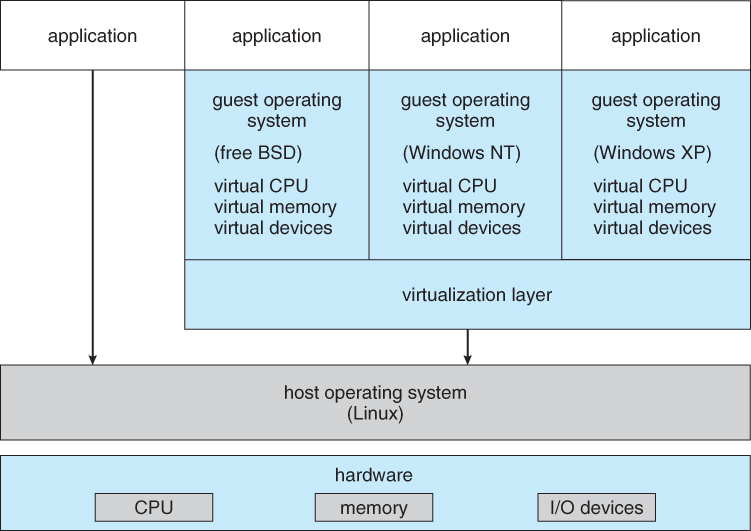
  • Abstracts the 80x86 hardware platform, allowing simultaneous operation of multiple Windows and Linux OSes, as shown by example in Figure 2.19:

Figure 16.9 - VMWare Workstation architecture
2.8.6.2 The Java Virtual Machine
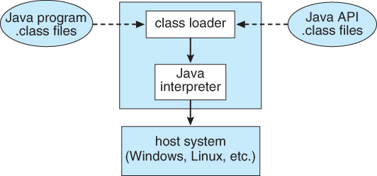
  • Java was designed from the beginning to be platform independent, by running Java only on a Java Virtual Machine, JVM, of which different implementations have been developed for numerous different underlying HW platforms.
  • Java source code is compiled into Java byte code in .class files. Java byte code is binary instructions that will run on the JVM.
  • The JVM implements memory management and garbage collection.
  • Java byte code may be interpreted as it runs, or compiled to native system binary code using just-in-time ( JIT ) compilation. Under this scheme, the first time that a piece of Java byte code is encountered, it is compiled to the appropriate native machine binary code by the Java interpreter. This native binary code is then cached, so that the next time that piece of code is encountered it can be used directly.
  • Some hardware chips have been developed to run Java byte code directly, which is an interesting application of a real machine being developed to emulate the services of a virtual one!

Figure 16.10 - The Java virtual machine
  • The .NET framework also relies on the concept of compiling code for an intermediary virtual machine, ( Common Language Runtime, CLR ), and then using JIT compilation and caching to run the programs on specific hardware, as shown in Figure 2.18:

Figure 2.18

Saturday, January 8, 2022

Data Warehouse is Really Different from a Normal Database

Don Jones differentiates the difference between a normal database and a data warehouse in a concise and precise manner in following bullets:
An operational data store (ODS), which you may also call an Online Transaction Processing (OLTP) or transactional database, has several key features:
  • It contains detailed information. For example, it not only contains summary information such as the total amount of an order but also detailed information such as how much each item costs.
  • It is designed to process transactions, meaning it’s typically dealing with one piece of data at a time: one order, one product, one customer. It may be used to generate basic reports from this data, but it’s structure is optimized to support rapid access to small chunks of data.
  • The schema is rigid and unchanging.
  • It contains up-to-date information, and is updated in real-time.
  • The quality of input data is often very high, meaning applications and other elements ensure that correct data goes into the data warehouse.
A data warehouse, in contrast, often includes these features:
  • Some data may be summarized, meaning detail is not available. You may be able to tell the total amount of a given order but not the cost of each product contained in the order.
  • Its purpose is to drive analysis and decisions. Access is usually for large quantities of data, in order to see trends.
  • The schema may be loosely structured and may change over time to support different analysis scenarios.
  • The information is historical and may not be entirely up to date. The emphasis is on past data and trends, more so than immediate, real-time data.
  • Data is often “cleaned,” meaning errant or “edge” data may be removed to make trends clearer. Data warehouses tend to focus on sets of data rather than on individual elements.
Companies with a data warehouse will always have one or more “normal” databases that feed the data warehouse.
(Source: http://nexus.realtimepublishers.com/content/?tip=how-is-a-data-warehouse-really-different-from-a-normal-database)