Plotting

• The following images were captured from a visualization of a distillation tower developed for a CAVE VR system:

• 
  

Commands and Techniques Common to All Plot Types

• Generate data in Matlab or load in a data file generated externally
  • Use the colon operator as needed to extract subsets of data, e.g. columns.
  • Cropping a plot - Data values of "NAN" ( Not a number ) are not plotted.
  • Plotting from the Workspace
    • Right-click on one or more data items and select a plot type from the pull-down menu
    • When selecting multiple data items, the order of selection is important.
    • The commands generated are displayed in the command window - Use help or doc to learn more about them, and copy them into scripts as necessary.
  • Plotting using plotting commands
    • Any of the plot commands can be issued in the command window or from a script.
  • Porting plots to other documents, e.g. to include in a written report
    • From plot window, select "File, Save As", and select a file type compatible with your other program, e.g. jpeg
  • Annotating plots
    • title - Places a title on a plot
    • xlabel, ylabel, zlabel - Labels the axes of a plot
    • text( x, y, 'text' ) - places text at the coordinates specified
    • gtext - places the text interactively using a mouse and cross hairs.
    • grid - "grid on;" or "grid off;" to display a background or not.
    • legend - For multi-line plots
    • axis - off, equal, image, tight, limits
      • The "axis" command can also be used to adjust the scaling ( but not the values ) of the axes.
    • colorbar - shows the mapping of numbers to colors
  • Most plotting commands will use row and column numbers to label the axes if no alternative data is provided.
    • There is generally a variation that allows you to provide your own data for labeling the axes.
    • Example: pcolor( x, y, data ) instead of pcolor( data ), where "data" is a 2-D matrix and "x" and "y" are vectors equal in length to the number of columns and rows respectively in the data matrix.
  • subplots
    • subplot( m, n, p ) sets up to plot in position "p" of an "m" row by "n" column grid of plots.
    • "p" increases row-wise, so 1 to n on the top row, n+1 to 2n on the second row, and so on.
    • The position p may span multiple cells, e.g. subplot( 2, 3, 5:6 ); or subplot( 3, 3, [2,3,5,6] );
    • For style purposes, indent plotting commands under a subplot command.
  • colormaps - controls mapping of data values to colors for many plot types
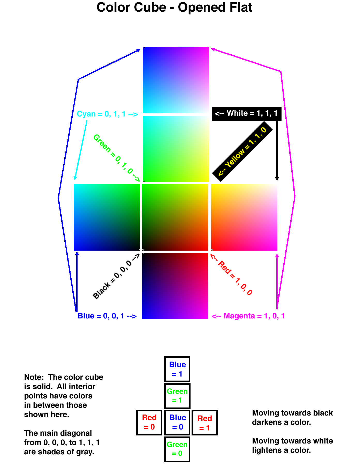
    • A "color" is a set of 3 numbers, indicating the relative amount of red, green, and blue light.
      • The color cube is one good explanation of how the three primary colors combine to make any combination
        • red + green = yellow ( 1, 0, 0 + 0, 1, 0 = 1, 1, 0 )
        • red + blue = magenta ( 1, 0, 0 + 0, 0, 1 = 1, 0, 1 )
        • green + blue = cyan ( 0, 1, 0 + 0, 0, 1 =0, 1, 1 )
        • black = 0, 0, 0; white = 1, 1, 1; Any color with red = green = blue is a shade of gray
        • Orange is half way between red ( 1, 0, 0 ) and yellow ( 1, 1, 0 ). So orange = ( 1, 0.5, 0 )
        • Pink is halfway betwen red( 1, 0, 0 ) and white ( 1, 1, 1 ), so pink = ( 1, 0.5, 0.5 )
        • A line from red to black passes through maroon and then brown
    • A colormap is any array of 3 columns and any number of rows, representing an array of colors.
    • "help graph3d" for list of pre-defined colormaps and other useful 3D graphing commands.
    • Pre-defined - Gray, copper, pink, bone, hot, cool, jet, hsv, spring summer, autumn, winter, lines
      • e.g. "colormap gray;"
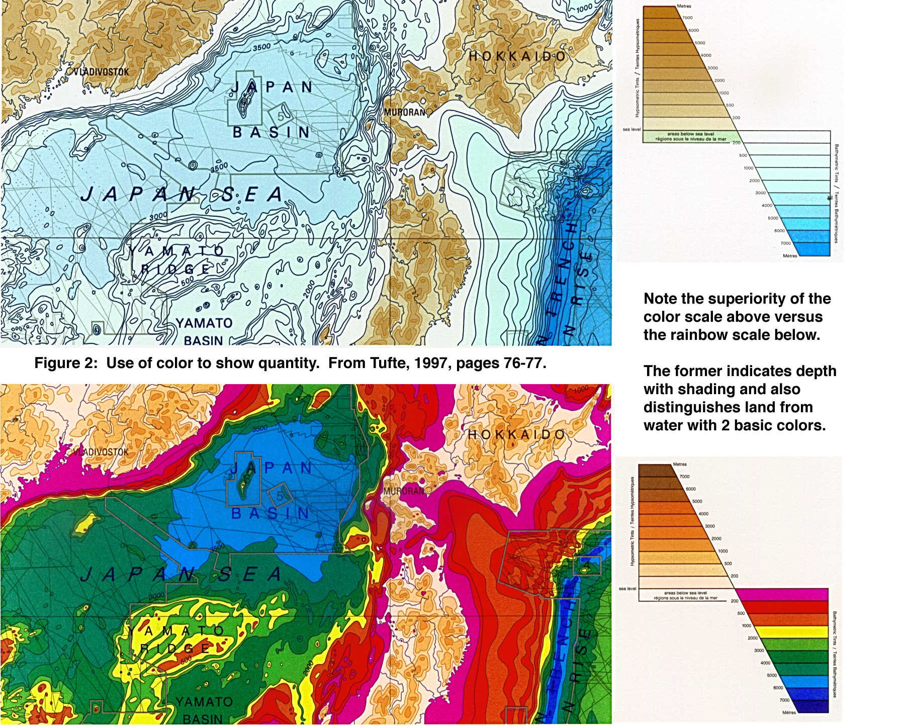
    • Edward Tufte presents an excellent example of the difference between good and bad color mapping.
    • User-defined - Any matrix of 3 columns of RGB values, in the range 0 to 1.0 inclusive.
      • See sample script colormaps.m
    • Display with rgbplot
    • Note: Colors can either be represented as integers ranging from 0 to 255 or floating point numbers ranging from 0.0 to 1.0, and Matlab can sometimes use either one, so it is sometimes necessary to convert from one data type to the other. ( E.g. im2double converts an image file from unsigned 8-bit ints ( uint8 ) to doubles.
  • Subimage: There is a problem trying to display multiple images with subplot if the images use colormaps, because a single figure can only use one colormap. You can get around the problem by using subimage, ( withtin subplot ), which converts the images to true color, eliminating problems with colormap conflicts.
  • Multiple plots on a common set of axes
    • plotyy - Creates 2 y axes, one along the left edge and one along the right
    • hold - Toggles whether the current plot is held for future plotting commands. ( Used for plotting multiple plots of different types on a single set of axes, such as a line plot and a bar chart for example. ) Can also be used as "hold on" and "hold off".
      • "plot" can also plot multiple lines on the same set of axes, as can many other plotting commands.
    • figure - Create a new figure, make a particular figure active, or bring up the current figure.
      • e.g. figure( gcf );
  • Line Specifications - line types, colors, markers, etc.
    • Given as a text string of special characters. For example, "plot( x, y, 'ro' );" plots the x y data using a red line ( 'r' ) and circles as data markers ( 'o' ).

2-D Plots

• Common 2-D plot commands
• plot - Basic line plots
• plotyy - Plot multiple plots using two Y axes, one on each side
• polar - Polar coordinate plot
• loglog, semilogx, semilogy - logarithmic plots
• errorbar - Plot error bars along a curve, not necessarily equal.
• bar, barh - Bar plots, vertical or horizontal
• pie - Pie charts
• hist - Histograms
• contour - Contour plots. ( See also surfc below. )
• comet
• feather - Vectors distributed along a line.
• quiver - Vectors distributed over a 2-D field, e.g. wind directon & strength.

3-D Plots

• Common 3-D plot commands
• plot3, comet3, bar3, quiver3, contour3, etc.
• surf, surfc
• pcolor
• Shading:
• Shading flat - every polygon is a solid color, with no lines at polygon borders.
• Shading faceted - As flat, with black line borders.
• Shading interp - Each polygon has a range of color values, smoothly varying from one corner to the next.
• ( Pcolor ignores the last row and column of data with flat or faceted shading, but uses the values with interpolated shading. )
• "view(az,el)" will set the viewpoint for a 3-D graphs as the azimuth ( polar angle in the x-y plane ) and elevation ( angle above the x-y plane ) given.

Images

• imshow ( Image Processing Toolkit )
• imagesc ( basic Matlab )